
PL computations showed a memory leak, ending up in problems during fitting with frequent re-computations of the model. The leak has been fixed today.
Category Archives: SCOUT
New ‘News’ command
The function of the menu item ?/News has been changed – it opens this documenation of program changes now.
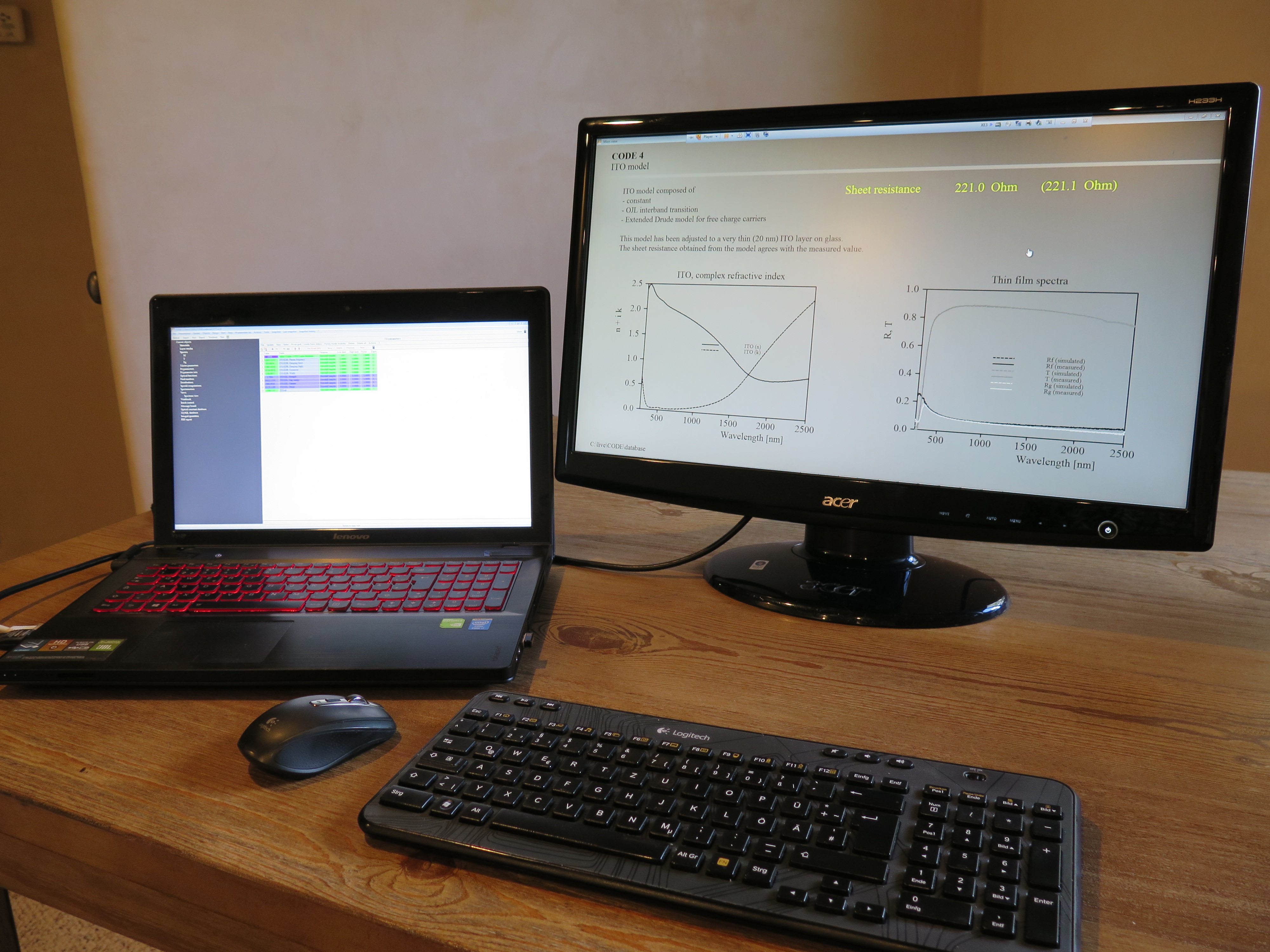
Working with a separate main view window
We are in middle of the transition to object generation 4.xx which will be delivered with a lot of useful program configurations (and a guide of the user to easily find what is needed). Some of the new configuration files come with explanations in the main view, telling the user what to do in the treeview.
In order to efficiently work with such configurations it is useful to see both the main view and the treeview at the same time. This is now possible with the command ‘Actions/View/Open external view’ which opens a separate window showing the main view. Ideally you push this window to a second monitor (if you have one). Here is an example:
Several bugfixes
We have removed an irritating “feature” which had caused some trouble in the past: If you worked with KKR susceptibilities and had already selected some of the interband transition parameters as fit parameters, it was not possible to insert new interband models before the existing ones without doing damage to the configuration. It was also not allowed to change the order of interband transition models. These restrictions have been removed.
It was also possible to delete an item inside a KKR susceptibility although a parameter of this item was selected as fit parameter. This caused access violation errors. This issue has been resolved as well.
Pressing F7 to switch from the treeview level back to the main view caused access violations in some cases (without doing damage – it was just annoying). This has been fixed.
Editing objects sometimes means to go through several user dialogs. The behaviour of the ‘Cancel’ button has been changed in some cases: It used to cancel the current dialog and jump to the next one – now a click on ‘Cancel’ shuts down the edit operation completely.
New ellipsometry import routine
Ellipsometry objects can now import data saved in *.pae files by SOPRA ellipsometers.
Although the angle of incidence is stored in such files the value of the angle of incidence of the ellipsometry object (which is used for the computation of simulated data) is not changed. This way you can import data measured at 70°, for example, and still do the computations for 69.9° – a small difference is sometimes necessary to correct for experimental uncertainties.
Updated import routine
The import routine for text files (xy-format) has been improved to allow to read data from files with several data columns. If you use this routine in batch operations or through OLE automation, you can now specify the column to read from as input option. Option = 1 means to read from the first column, option = 3 reads from the 3rd.
XRR computations
The list of spectra in SCOUT and CODE offered object types called ‘Angle scan’ and ‘XRR’ for a long time already. Although the names indicate what these objects are made for, there was no documentation up to now. We have started to update the SCOUT help with respect to these objects.
Here are the links to the relevant sections:
Improvement of Gervais oscillators
Certain parameter combinations of Gervais oscillators may lead to unphysical optical constants (i.e. negative imaginary part of the dielectric function). Physical meaningful solutions satisfy a sum rule for the damping constants which may be used to steer the fit into the direction of ‘good’ solutions.
The “check sum” (sum of the difference of LO damping and TO damping for all oscillators) can now be obtained as optical function. Use the optical function “my_material (Gervais_condition)” to retrieve the current value of the check sum.
In order to make use of this number in a fit you can proceed like this(this hint will work in CODE only): Generate an integral quantity of type ‘function of int. quant.’ and call it ‘Gervais check sum’. As formula to compute the value use the term “of(1)” (here it is assumed that the check sum is the first optical function). So the integral quantity is the check sum itself.
Now define a penalty shape function for this integral quantity. It should be 0 if the check sum is positive, and get large for large negative values of the check sum. An expression like “abs(y)*step(-y)y)” will do the job (in penalty shape functions for integral quantities the symbol “y” refers to the current value of the integral quantity). This way large negative values of the check sum are severely punished whereas positive values do not contribute to the fit deviation at all.
Finally activate the option “Combine fit deviations of integral quantities and spectra” in the fit options dialog (File/Options/Fit). This lets CODE simultaneously minimize the difference of measured and simulated spectra and the fit deviation of the integral quantities (which is in this case the penalty for an unphysical check sum). Eventually you have to experiment a little bit with the weight of the ‘Gervais check sum’ in the list of integral quantities in order to get a good fit.
Bugfix Gervais oscillators
Using several Gervais oscillators at the same time eventually caused numerical problems. This has been fixed today – you can now really use all 10 oscillators which are offered by the “Gervais dialog”.
Import routine for TohoSpec3100 added
Reflectance spectra of the TohoSpec3100 system can now be imported both in SCOUT and CODE.