CODE 3.98
The capabilities of ‘parameter variation’ objects in the list of special computations have been enhanced. You can now define ‘offset functions’ which are computed once before the parameter variation is executed. The example below discusses an application of this feature.
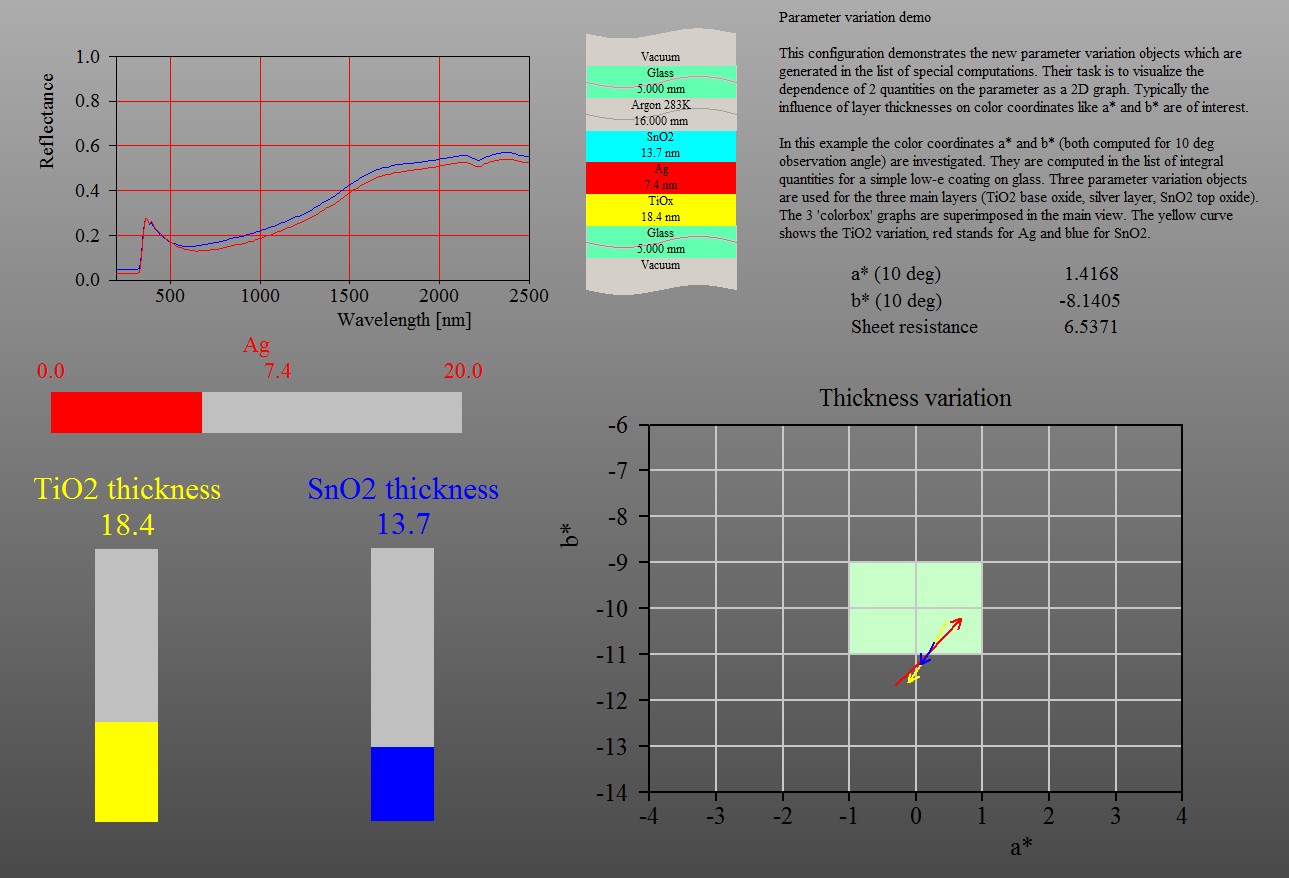
Suppose you are computing the dependence of color coorinates a* and b* on layer thicknesses. For each layer you generate an ‘arrow diagram’ showing how the position of the layer stack in the a*-b*-plane changes with thickness modifications. Superimposing 3 of such diagrams would give a graph like this:
 Unfortunately the model does not perfectly reproduce the measured reflectance spectrum. As a result, the ‘measured’ color position is different from the simulated one. In this situation you might want to display the arrows at the ‘measured’ color position, believing that the direction and the size of the arrows will be similar there. A graph like this would show operators where they are with their real product and where they would go with thickness variations.
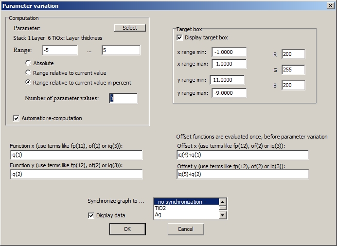
You can generate the desired offset the following way. Compute a* and b* of the simulated spectrum in the list of integral quantities as item 1 and 2, and compute the a* and b* of the measured spectrum as items 4 and 5. In function definitions you can refer to these numbers as iq(1), iq(2), iq(4) and iq(5), respectively. The dialog for the first parameter variation object (modifying the TiO2 layer thickness) would look like this:
Defining similar offsets for the other two layer thickness variation objects you will get a shifted arrow graph, centered at the color position of the measured reflectance:
 Obviously, you should use this feature only in cases where you are sure that the applied offset is justified and does not lead to wrong conclusions.