Category Archives: Computing and fitting spectra

Variation of 2 model parameters

We have updated the list of special computations. You can now do variations of 2 parameters rather easily, using objects of type ‘2 parameter variation’.

As an example we use a low-emission glass coating with several layers:

The goal of this exercise is to learn how the average transmittance in the visible (light transmittance) depends on the thickness values of the TiOx and SnOx layers. In our example configuration, the light transmittance is computed as third integral quantity:

To do the required computations we generate an object of type ‘2 parameter variation’ in the list of special computations:

Editing the new object brings up this dialog:

For each parameter you can select which one it is and how the range of values is chosen. The editor ‘Function to be evaluated’ allows to enter the quantity you want to compute for each pair of parameter values – in our case this is iq(3) (the light transmittance). If you check the option ‘Automatic export to workbook after computation’ the obtained data are written to the workbook.

Once this dialog is closed another one opens which is used to set graphics parameters for the graph of the data. This graph can be shown in a view if you drag the special computation object to a list of view items. The first parameter (TiOx in our case) will be displayed on the parameter axis, the second parameter values (SnOx thickness) will be displayed along the x-axis:

Please note: Computations may require some time for this type of object. Automatic updates are switched off which means you have to actively trigger the computation. You can do that in the list of special computations by selecting the object and then click the ‘Update’ menu item. If you display the object in a view re-computation is triggered by a click on the view object. Be careful to click only when you really want to start a new computation!

The graph looks like this:

You can also select to generate false color plots which you can use to display a kind of contour graph:

As mentioned above you have the option to store the computed data to the workbook. If your object is called ‘LT chart’ a workbook page with this name is created and the data are written to the worksheet, including minimum and maximum value as well as the position of these extrema:

CODE: Using measured sheet resistance values in batch fitting

Besides optical spectra CODE computes sheet resistance values of layers stacks. A sheet resistance object in the list of integral quantities computes the current value and – with the ‘Optimize’ option turned on – the squared difference to a given target value.

If you type in a measured sheet resistance value as target value CODE optimizes a layer stack to reproduce measured electrical performance (only if the option ‘Optimize’ is switched on, of course). If you check the option ‘Combine fit deviation of integral quantities and spectra’ (File/Options/Fit) you can fit spectra and sheet resistance at the same time, balancing importance by setting proper weights for each quantity.

We have now added the ability to take into account measured sheet resistance values to batch fitting. In order to use this new feature you have to define a sheet resistance object in the list of integral quantities and name it ‘sheet resistance fit’. Set its ‘Optimize’ option ‘On’. Then generate a new batch fit based on the current model – or use an existing one. Here is an example of the results page:

Note the empty line between the last spectrum (‘Reflectance’ in this case) and the line called ‘Fit’. Enter the key phrase ‘sheet resistance fit’ into the first column and type in or copy the measured values for each sample (i.e. for each column). The table should look like this now:

That’s all – you are now ready to start batch fitting. For each sample the measured values will be entered as target values and CODE will optimize both spectra and sheet resistance values.

You might encounter the difficulty that measured and simulated sheet resistance values do not easily agree. In this case you should check if your sample might show a depth gradient of the conductivity. A reason could be a depth dependent density of defects like grain boundaries within the layer. In such a case you should consider dividing the conductive layer into several parts with different damping constants of the charge carriers. You can read a discussion for silver and other conductive layers here.

More on error messages …

Object generation 5.30 comes with some more script functions supporting error handling. We have generated a simple demo application in CODE which looks like this:

While some measurement routines (list of spectrometers) and other procedures produce error messages by themselves you can generate error message by a script command:

  • raise error message,0,1,This is wrong – user tried do divide by 0
  • raise error message,0,2,This is a warning only ..

Here the first integer parameter indicates the type of error, the second one the classification. ‘1’ means ‘critical error’, ‘2’ stands for warning.

The script command ‘verify function value’ automatically raises an error message if the condition the function value is out of range. You can add the keyword ‘silent’ to suppress a dialog popping up – in this case the classification is ‘Warning’. Without the keyword you get a dialog and classification ‘critical error’:

  • verify function value,of(1),0.3,0.4,reflectance maximum,silent
  • verify function value,of(1),0.3,0.4,reflectance maximum

Error messages get a timestamp and are collected in an array until the script command ‘clear error messages’ is executed.

If you use CODE to acquire spectra with a spectrometer object you can generate measurement reports which collect all measured spectra for a sample – these are JSON files. Should there be warnings issued by the measurement scripts the corresponding error messages are stored in the ‘error section’ of the JSON files as well.

The new view element ‘error messages view’ shows error messages in a view.


How to develop flexible optical constant models based on given n and k tables

Materials used in thin films may differ in their optical constants n and k from the corresponding bulk versions. Even if you find optical constant tables in literature for your application you may need to make some adjustments to the n and k values. This is certainly difficult if you have just a table of fixed values – what you need is a flexible model which can adjust the spectral shape of n and k by modifying a few key parameters only. This short tutorial shows how to proceed in such a case.

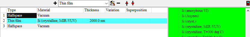
Crystalline silicon is used as example. The database of our SCOUT and CODE software packages contain several silicon versions. Here I have selected the item ‘Silicon (crystalline, MIR-VUV)’. These are the n and k data, featuring several interband transitions and a slow decay of k towards the indirect band gap around 1.1 eV:

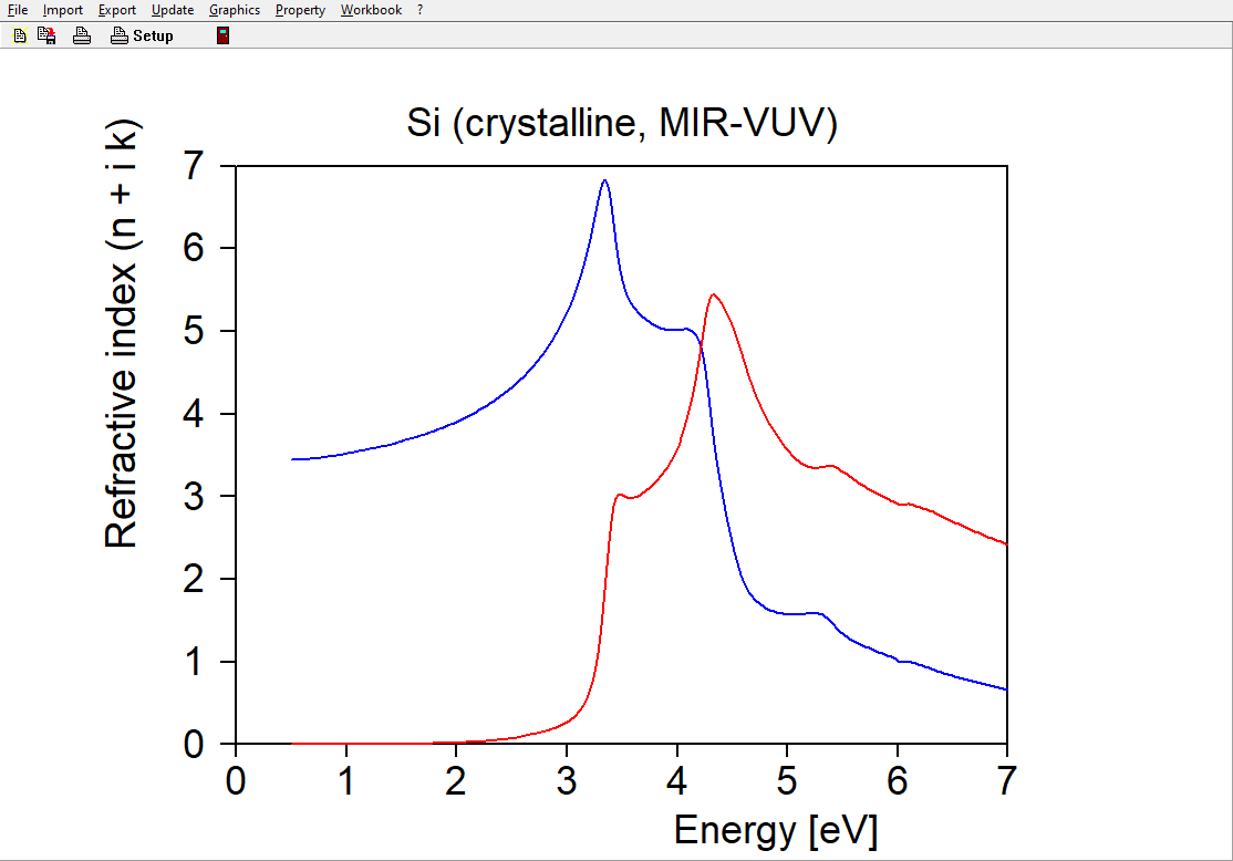
If you change the temperature of a silicon wafer or deposit poly-crystalline silicon thin films you may observe similar structures but not exactly the same n and k – a flexible model would be nice to have. Our strategy to develop such a model will be this: First, we generate ‘measured data’ which are computed using the existing n and k table values. Then, in the second step, we setup a suitable model and adjust its parameters to reproduce the ‘measured’ data. If the ‘measurements’ provide enough information the n and k values of the model should be almost the same as those of the original table.

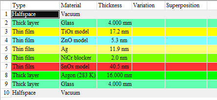
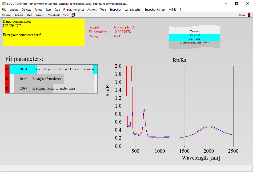
Since we will simulate the measurements we can easily work with a system which would be almost impossible to realize. In order to clearly ‘see’ the weak silicon absorption in the visible we use a 2 micron thick free standing layer – this layer is quite transparent and it will generate a nice interference pattern. To match the amplitude of the fringes will be difficult with wrong k values – so this setup ensures good n and k data of the model in the visible and NIR. The layer stack is this:

Using this layer stack we could now generate several reflectance and transmittance spectra, taken at various angles of incidence. This would make a nice set of ‘measured data’ for the fit procedure. However, to make our life as easy as possible we can use an ellipsometry object in the list of spectra. Objects of this type have the option to compute so-called ‘Pseudo n and k’ values. With this option the ellipsometric angles Psi and Delta are represented by pseudo n and k values of a virtual single interface. In spectral regions where our silicon layer is opaque the pseudo n and k values are the same as the real ones. In the transparent region the pseudo n and k values reflect the interference structures – this looks strange, and one could certainly question the usefulness of the concept ‘Pseudo n and k’. However, the interference pattern is what we go for to get good small k values in the model. The blue curves below show the generated pseudo n and k values. Within this example we will work in the spectral range 200 … 1000 nm:

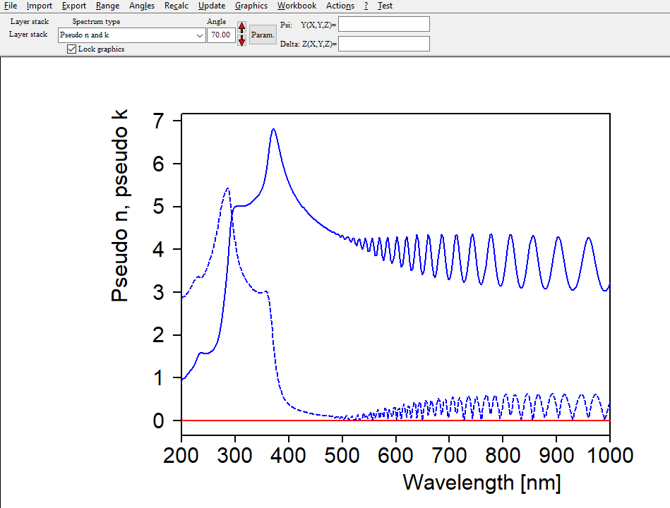
Ellipsometry objects offer the local menu command ‘Actions / Use simulated data as measured data’ which is what we need now. The blue curves are now copied to the red measurement data as if we had imported measured data.

We can now replace the material object by our first model in the layer stack. I have started with a very simple model which consists of a constant real part of the refractive index and a Tauc-Lorentz model (inside a KKR susceptibility object). It is a good idea to generate a new item of type ‘Multiple spectra view’ which can show both the original table values of n and k and the model values in one graph (lower left side). With this simple model, you cannot expect a good match since  silicon shows several interband transitions in the range 200 … 1000 nm:

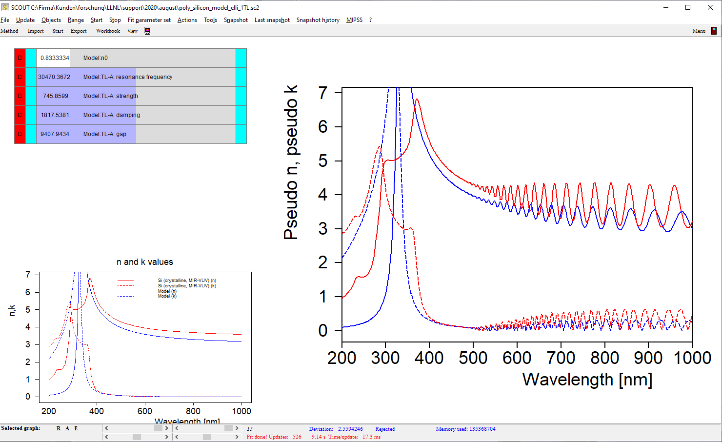
However, if we limit the range to 400 … 1000 nm the simple model works quite well:

For the full range (200 … 1000 nm) we need more interband transitions. Sticking to the Tauc-Lorentz oscillator type, I have added 2 more which brings up to a new level (still not satisfying, though):

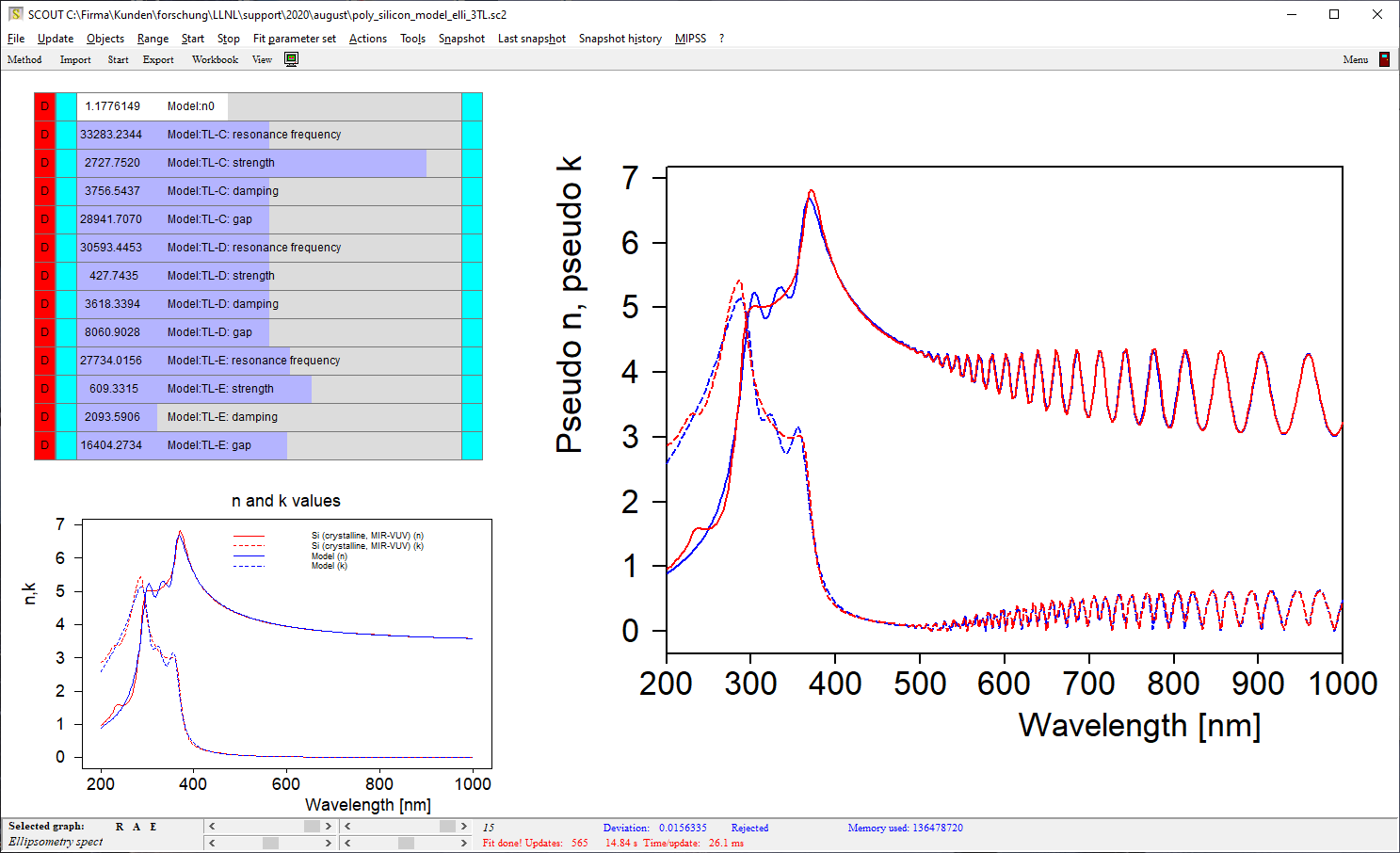
Depending on your patience (and the needs of the final application) you can add more features as you like, approaching the former table values of n and k more and more. I stopped my example at this level:

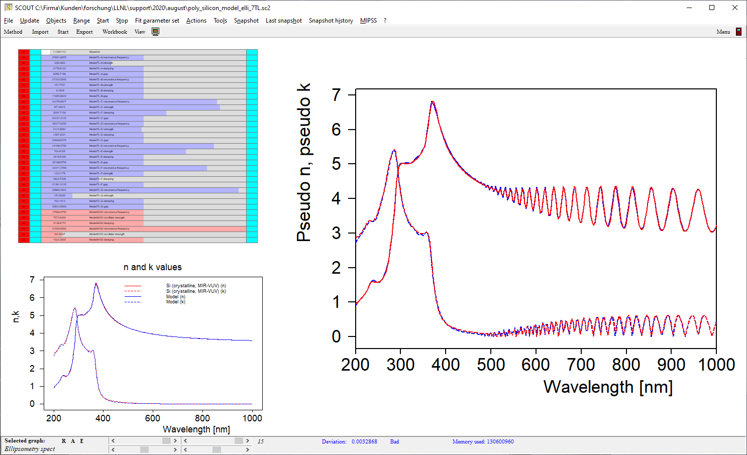
The model developed for silicon this way can now be saved to the optical constant database for future use. You can use it for studies of systematic variations of deposition conditions and generate tables like ‘resonance frequency vs deposition temperature’.

You can follow the strategy shown in this tutorial for all kinds of materials, as long as you get good tabulated values of n and k to start with.

Fit parameter sets embedded in configuration file

Starting with object generation 5.12, you can store fit parameter sets in a list called ‘Fit parameter pool’.  This list is stored as part of the SCOUT or CODE configuration file. Using fit parameter sets from the pool avoids the necessity to load them from separate files.

Instead of specifying a filename for the fit parameter set (which is still possible) you can use phrases like ‘pool(step 1)’ or ‘pool(oscillator strengths only)’ to load fit parameter sets with names ‘step 1’ or ‘oscillator strengths only’.

Using file based fit parameter sets is possible after all, of course.

Angle of incidence distribution

Spectroscopic experiments can never realize single angle of incidence but have to work with a (continuous) distribution of angles. Although in most cases the assumption of a single angle of incidence is a very good approximation there are cases where we need to take into account more details in producing simulated spectra. One example is taking reflectance spectra of small spots with a microscope objective, using a large cone of incident radiation.

For a long time our software packages can compute spectra averaged for a set of incidence angles, each one defined by the value of the angle and a weight. We have now implemented new features to simplify work in this field.

If you have prepared a list of angles of incidence you can now connect these angles to the angle of incidence that you have defined for spectrum object which owns the list of angles. You can check the option as shown here:

If you have activated this option you can use a set of angles with positive and negative values (centered around 0) as shown here:

If the angle of the parent object is 50° the computation of the spectrum is done for the 3 angles 45°, 50° and 55°, with weights 0.3, 0.4 and 0.3, respectively. If you have declared the angle of the parent object to be a fit parameter the set of 3 angles is moved automatically when the value of the center angle changes during the fit. This helps to adjust the distribution of angles to match the experimental settings.

Finally, there is a new fit parameter called ‘Scaling factor of angle range’. This number scales the distance of the individual angles to the center angle: If the factor is 1.0 the original angles are used. If the factor is 0.1, for example, a value of 5° becomes 0.5°. Varying the factor between 0.1 and 2 in the example shown above, you can compute spectra for a distributions between -0.5° … 0.5° to -10° … 10°.

We hope that this new flexibility helps to achieve better fitting results for spectra measured with microscopes or other systems with spectra features depending critically on the angle of incidence.