The dialog that sets the parameters for ‘rating’ has been updated in object generation 5.12.
‘Rating’ is the transformation of the fit deviation (a floating point number) to a text-based category like ‘Good’, ‘Bad’ or ‘Perfect’.

The dialog that sets the parameters for ‘rating’ has been updated in object generation 5.12.
‘Rating’ is the transformation of the fit deviation (a floating point number) to a text-based category like ‘Good’, ‘Bad’ or ‘Perfect’.
Spectroscopic experiments can never realize single angle of incidence but have to work with a (continuous) distribution of angles. Although in most cases the assumption of a single angle of incidence is a very good approximation there are cases where we need to take into account more details in producing simulated spectra. One example is taking reflectance spectra of small spots with a microscope objective, using a large cone of incident radiation.
For a long time our software packages can compute spectra averaged for a set of incidence angles, each one defined by the value of the angle and a weight. We have now implemented new features to simplify work in this field.
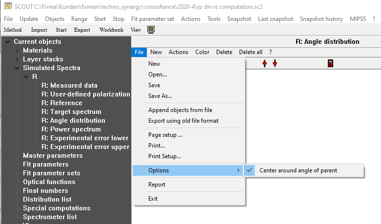
If you have prepared a list of angles of incidence you can now connect these angles to the angle of incidence that you have defined for spectrum object which owns the list of angles. You can check the option as shown here:
If you have activated this option you can use a set of angles with positive and negative values (centered around 0) as shown here: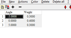
If the angle of the parent object is 50° the computation of the spectrum is done for the 3 angles 45°, 50° and 55°, with weights 0.3, 0.4 and 0.3, respectively. If you have declared the angle of the parent object to be a fit parameter the set of 3 angles is moved automatically when the value of the center angle changes during the fit. This helps to adjust the distribution of angles to match the experimental settings.
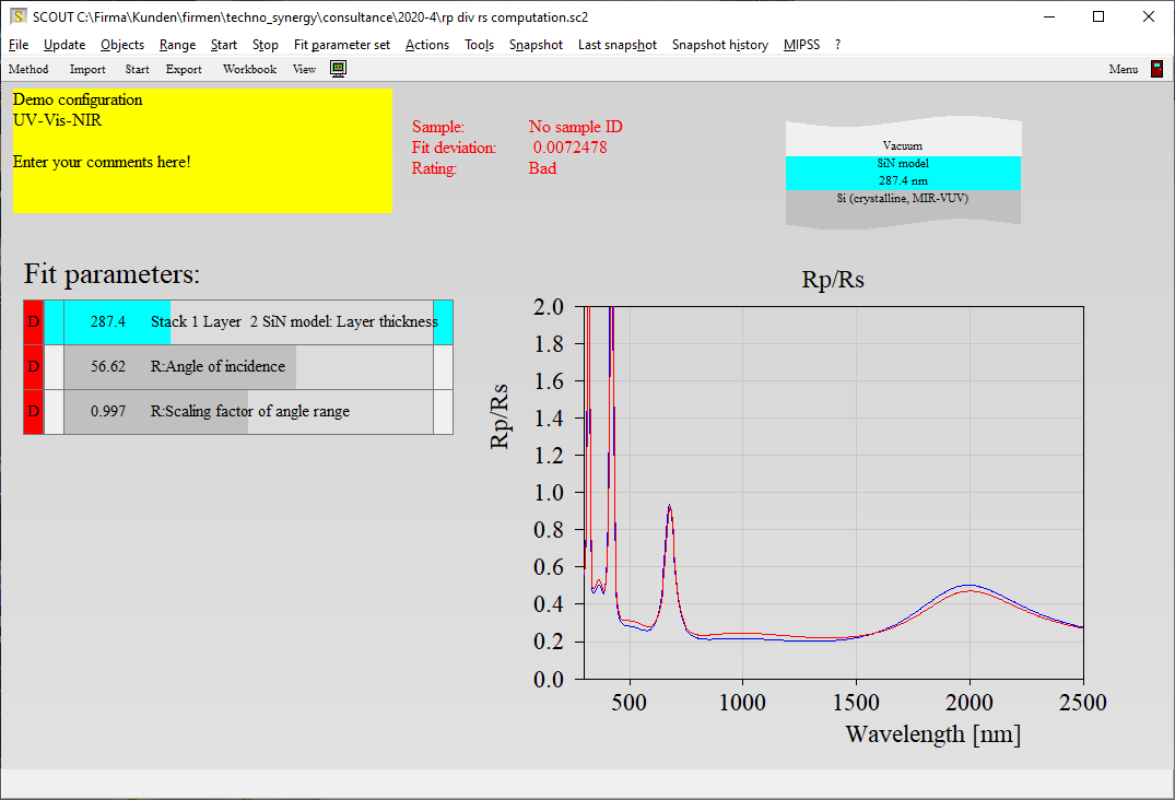
Finally, there is a new fit parameter called ‘Scaling factor of angle range’. This number scales the distance of the individual angles to the center angle: If the factor is 1.0 the original angles are used. If the factor is 0.1, for example, a value of 5° becomes 0.5°. Varying the factor between 0.1 and 2 in the example shown above, you can compute spectra for a distributions between -0.5° … 0.5° to -10° … 10°.
We hope that this new flexibility helps to achieve better fitting results for spectra measured with microscopes or other systems with spectra features depending critically on the angle of incidence.
Starting with object generation 5.11 we have introduced a new spectrum type called ‘Rp/Rs’. If you select this option the spectrum object computes the ratio of the intensity reflectance for p-polarized light and s-polarized light. This ratio can be directly fitted to experimental data if your measurement system produces this quantity as final result.
Having investigated a case where CODE stopped working after importing an older method, we found that a data field contained numbers marked as NAN (= not a number). Up to now we don’t know how this situation can arise – probably it was caused by a failing import of measured data.
The following mechanisms have been implemented to make the software survive this situation (active starting with object generation 5.09):
The BREIN cleaner tool now compresses complete product folders of the BREIN archive. This is done on demand, like it is possible for user-selected day or month folders.
The current day folder is compressed automatically as long as the cleaner tool is active.
Starting with object generation 5.05 the list of spectra offers a new object type called ‘Function fit’. It allows the user to define a function which may contain terms that retrieve optical functions, fit parameters and integral quantities (the latter in CODE only, but not in SCOUT). The function value is computed based on the current model and compared to a user-defined target value, or an interval of allowed target values. The fit deviation of the object is the absolute difference between current value and target value (or closest limit of the target range), taken to a user-defined power. If the function value stays within the target interval the deviation is zero.
Objects of this type can be used to impose restrictions to the model. If, for example, an optical function returns the real part n of the refractive index at a certain wavelength, you can define a target interval for n and generate a large deviation outside the target interval. This forces the fit to look for solutions that are compatible with the given range of refractive index values.
Design targets for color values or other integrated spectral values may not always be well-defined numbers. You can also search for designs where color values stay within tolerated boundaries, but it does not matter where exactly.
Such design situations can be handled in CODE using so-called ‘penalty shape functions’. However, the use of this concept turned out to be rather complicated.
We have now (starting with version 5.02) introduced a very easy definition of tolerated intervals for integral quantities: Instead of typing in the target value you can define an interval by entering 2 numbers with 3 dots in between, like ’23 … 56′ or ‘-10 … -8’. If the integral value lies within the interval its contribution to the total fit deviation is zero. Outside the interval the squared difference between actual value and closest interval boundary is taken, multiplied by the weight of the quantity.
Based on the WOSP-LEDO light source we have developed a spectrometer system that can be used to measure reflectance spectra in the wavelength range 270 … 900 nm. The light source is based on LEDs only.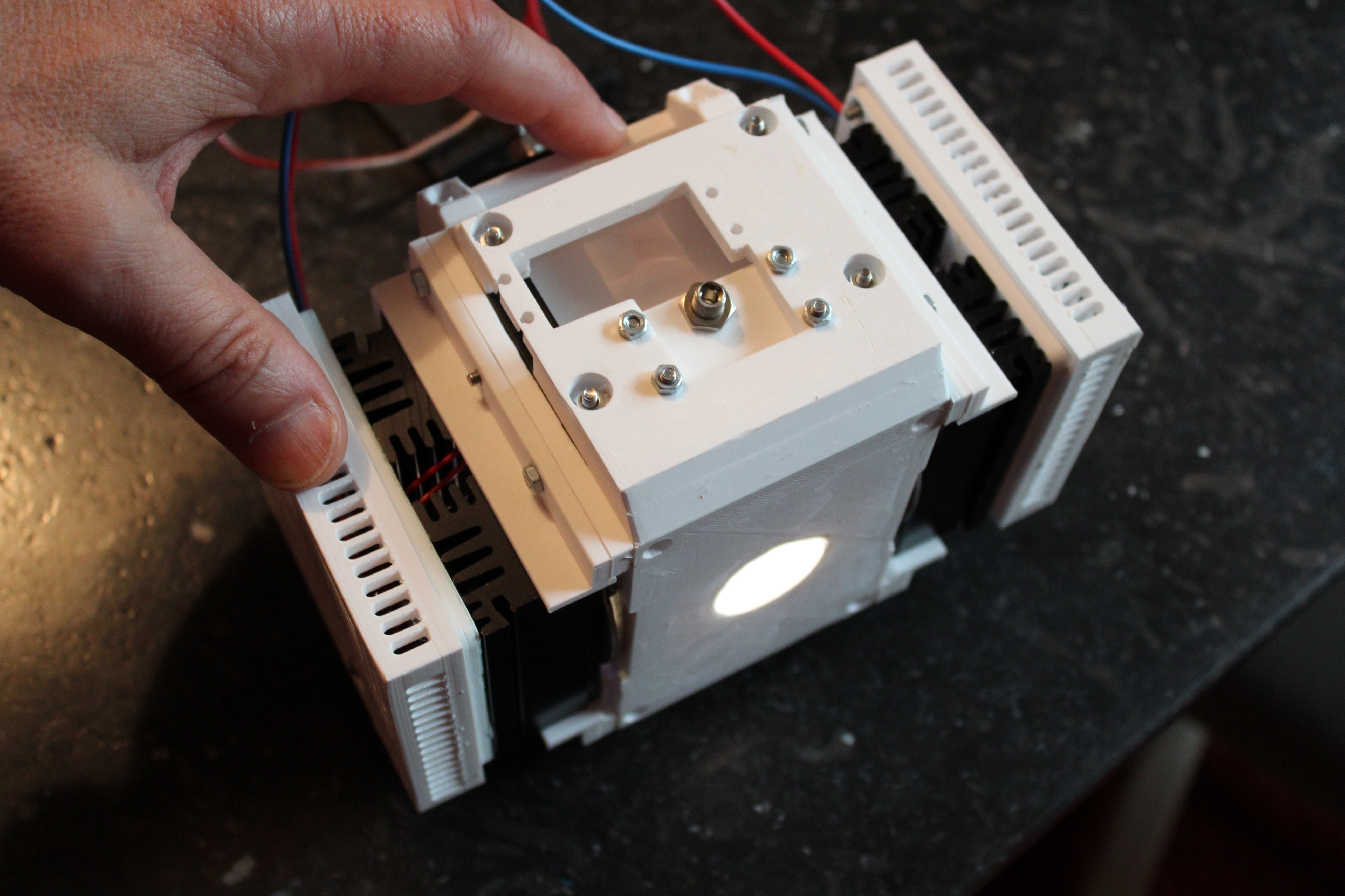
2 array spectrometers (not shown in the images) are used to record the sample signal and a reference signal at the same time. This makes the results independent of light source drifts.
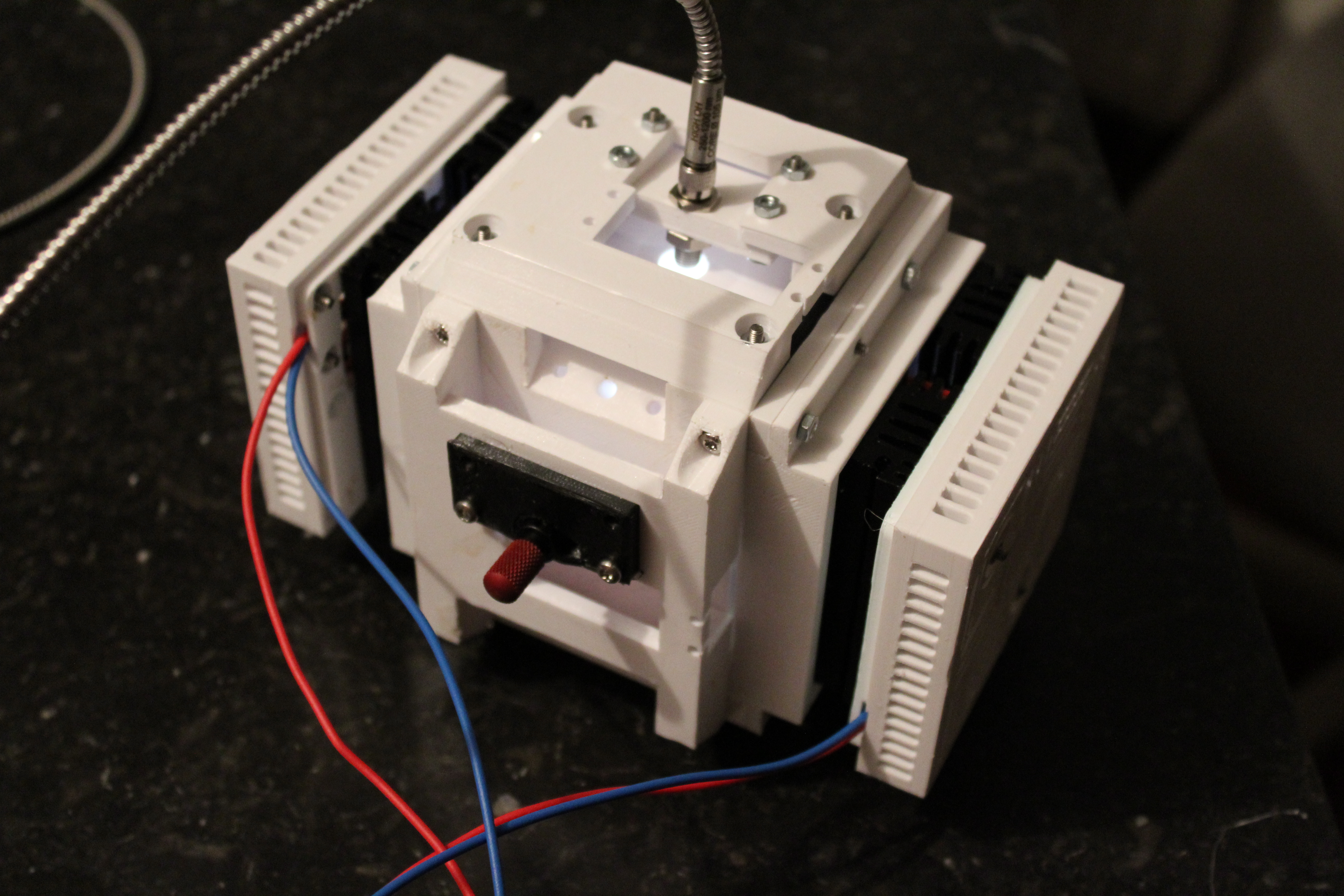
Samples must be positioned within a few mm distance to the sample port of the system. The measured spectra are tolerant against small sample tilts or height differences.
Spectral quality is the same as for WOSP-LEDO. The unit can be used as a light source for transmittance measurements as well.
The system requires an external power supply of 12 V DC.
We have implemented (starting with object generation 4.99) the Leng oscillator which has been developed to model optical constants of semiconductors. As shown in the original article (Thin Solid Films 313-314 (1988) 132-136) it works well for crystalline silicon:
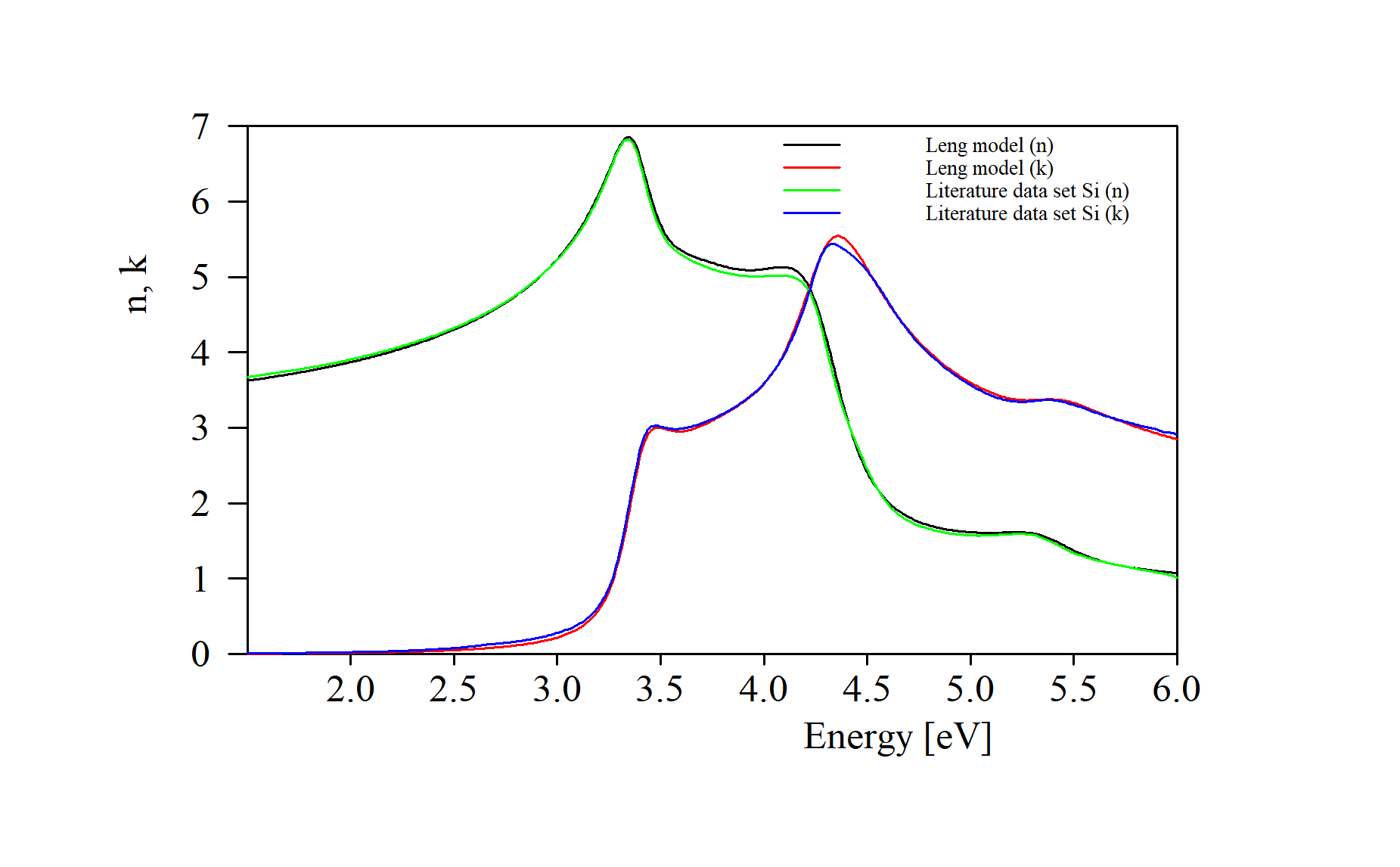
Warning: While the model works fine in the vicinity of strong spectral features (critical points in the joint density of states) it may generate non-physical n and k values in regions of small absorption.
Finally we have introduced a menu command (Actions/Delete selected record) to remove a record from the BREIN database. The action is – of course – password protected.