With CODE you can compute the photocurrent in an active layer of a solar cell. The photocurrent is available as integral quantity which can be the target of the layer stack optimization – very likely the target is ‘as high as possible’. Photocurrent objects make use of a special spectrum type in CODE which is called ‘Charge carrier generation’. Since the required steps to setup such a computational scheme are non-trivial (and a little bit hidden in the documentation) we have generated this tutorial which explains all details.

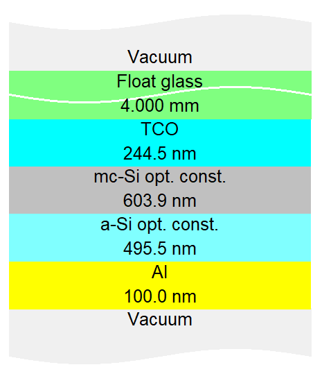
The example is a thin film solar cell with 2 active layers. One is micro-crystalline (mc-Si) and the other one amorphous (a-Si). Light enters through glass from the top. Between glass and the absorber layers a transparent conductive layer (TCO) collects charge charriers. The backside contact is made of aluminum.

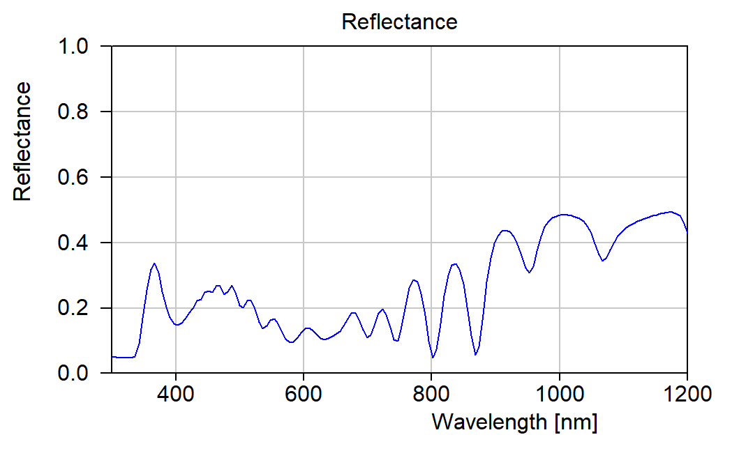
The reflectance of the stack is easily calculated – this is standard in CODE:

If you are interested how much light is absorbed in one of the active layers you have to generate a spectrum of type ‘Layer absorption’ in the list of spectra. Please note that this spectrum type works for layer stacks which consist of either ‘thick layers’ or ‘thin films’ – you should not have ‘rough interface’ or ‘thickness averaging’ layers in the stack.

‘Layer absorption’ objects require the selection of the active layer. A control element for this is available in the upper left corner:

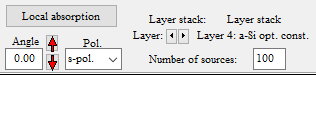
In addition, you have to set a parameter called ‘Number of sources’. CODE divides the layer of interest into several sublayers and computes the local electric field inside each sublayer. Then the absorbed power is computed and added up for all sublayers. ‘Number of sources’ is the number of sublayers – it should be selected high enough so that the final results do not change significantly if you change the number of sources somewhat.

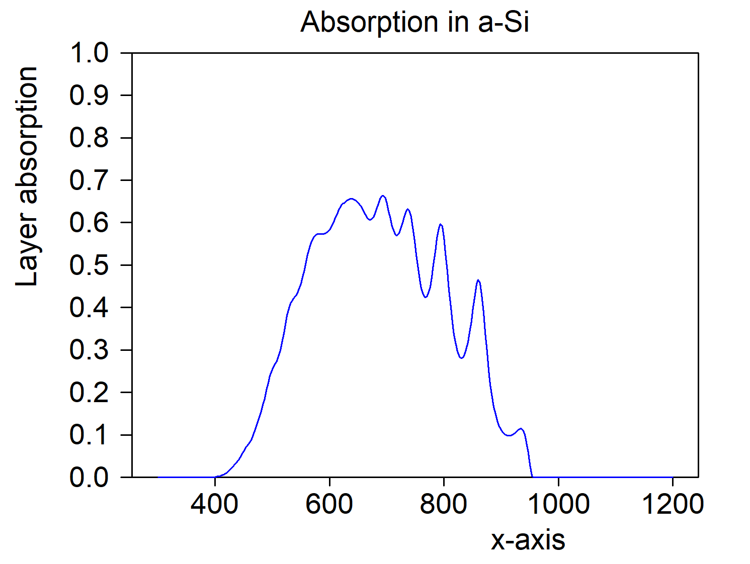
In our example the fraction of light absorbed in the a-Si layer is this:

What really counts for the performance of the solar cell is the number of electron-hole pairs generate by the absorbed light. Not every photon may generate an electron-hole pair that contributes to the current of the cell. The spectrum type ‘Charge carrier generation’ is used here: It works like the type ‘Layer absorption’ discussed above, but multiplies the absorbed fraction by an internal efficiency function.

Each spectrum of type ‘Charge carrier generation’ has subobjects called ‘Local absorption’ and ‘Generation efficiency’. The local absorption subobject shows the local absorption of light within the stack:

Starting at z=0 on the left we see the absorption within the Al layer, followed by the a-Si and mc-Si absorption. Finally, on the right side, the TCO absorbs in the UV and the NIR.

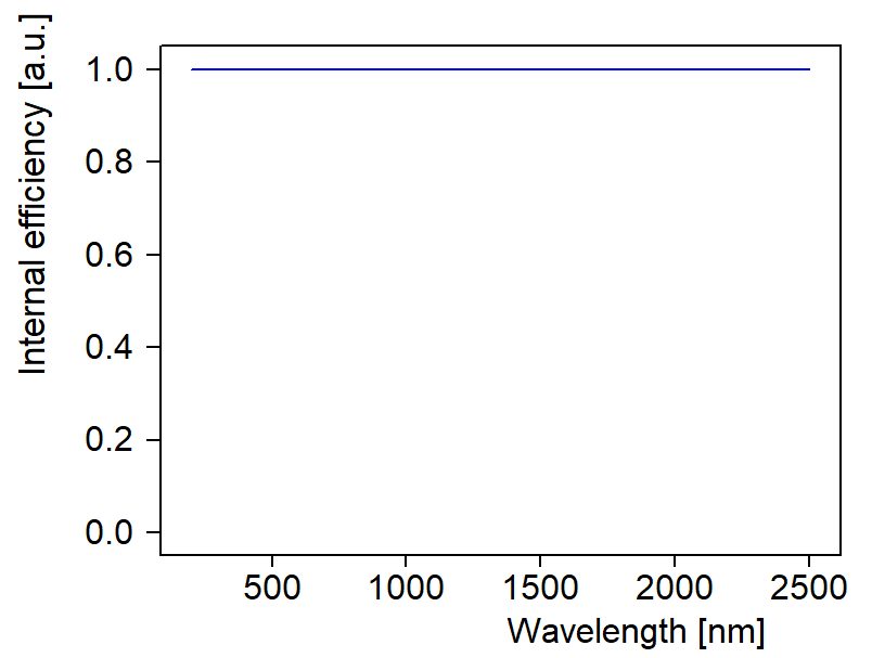
The subobject ‘Generation efficiency’ is used to define the spectral function that returns the probability of the generation of an electron-hole pair by the absorption of a photon. Per default setting the internal efficiency is one:

However, you can click on ‘Definition’ to open a list that allows more flexibility:

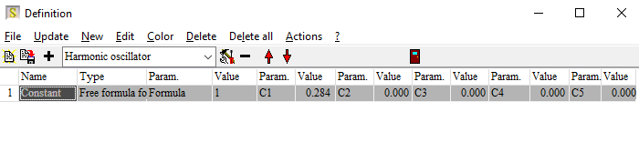In this list you can define a spectral dependence of the generation efficiency, using terms that you usually use for dielectric functions. You can use oscillators like this one:

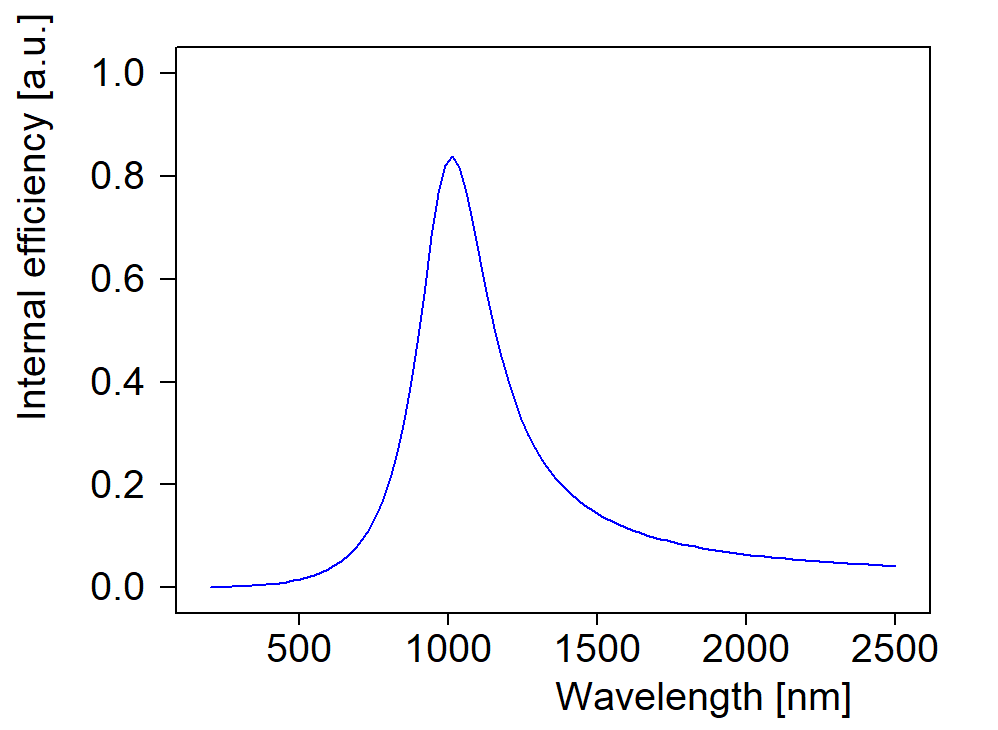
Or a superposition of many oscillators or any user-defined function. The parameters of each term show up as potential fit parameters – this allows to tune the model and get some information about the generation process.

For simplicity in this example the internal efficiency is 1.0.

Having defined ‘Charge carrier generation’ objects for both active layers (mc-Si and a-Si) CODE knows the relation of absorbed photons and generated electron-hole pairs for each wavelength. In order to compute a macroscopic property we have to integrate over the whole spectrum. This is done by objects of type ‘photocurrent’ in the list of integral quantities. For each active layer you have to define one photocurrent object and assign the proper spectrum:

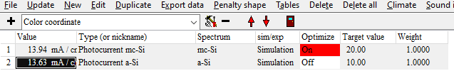
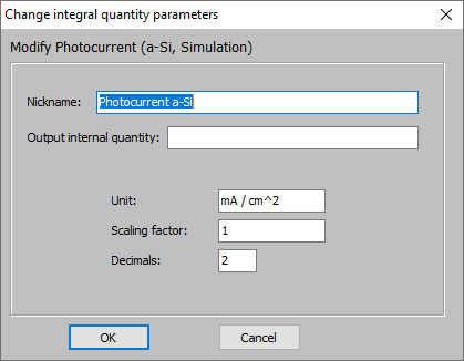
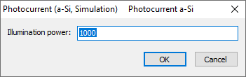
Editing a photocurrent object you can define the spectrum of the incident light and its integrated, total power. Please note that CODE uses the unit mA/cm^2 for the current density:

Next you have to define the spectrum of the incident radiation. Should the graph be missing press ‘Update’ to see it – or press ‘a’ on your keyboard for automatic scaling. Our example uses an AM1.5 spectrum. Do not worry about normalization – CODE will do that for you. You just have to provide the wanted spectral shape:

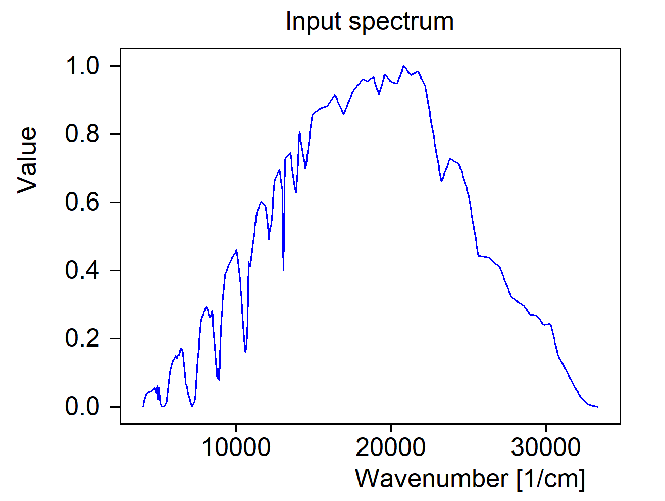
Finally, the total power of the illumination is entered in W/m^2:

Now CODE knows all parameters and computes the current density generated in the active layer.

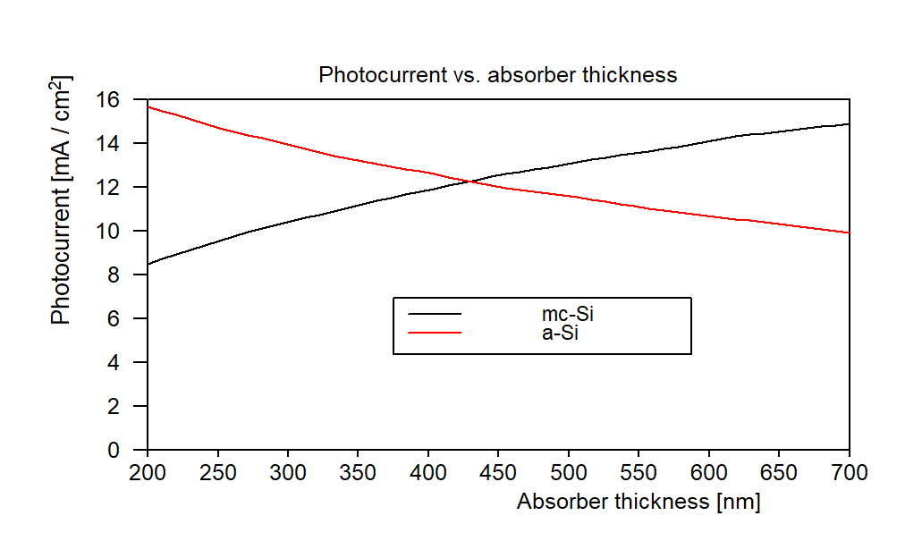
In our example we have 2 active layers which may have different layer absorption and also different current densities:

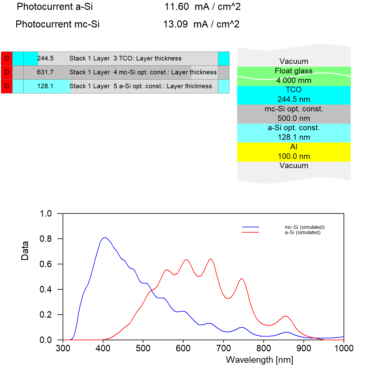
Depending on layer thickness values one or the other active layer produces more current. You can generate graphs like the following doing a parameter variation (which generates all data in the workbook) and a view element showing workbook data: