
There is a new video about ‘ bulk analysis’, i.e. doing optical fitting at high average speed using several instances of SCOUT and CODE in parallel.
Category Archives: Uncategorized
License changes
Times change, and the way we handle software licenses is changing, too. The info page has been updated recently (=today) – we are sure that for most users nothing will change in the way SCOUT and CODE are used.
Introducing MIPSS for parallel computing
Due to the nice competition of AMD and Intel computers with many cores become more and more affordable. Unfortunately, our software products SCOUT and CODE use only one core at a time up to now. In order to benefit from increased computing power of modern processors we have implemented MIPSS which means Multiple Instances for Parallel Spectrum Simulation.
MIPSS can be used to significantly speed up batch control computations. We have published a video tutorial that shows how to do this.
In addition, a new mechanism called ‘Bulk analysis’ has been implemented both in SCOUT and CODE. It is applied when a large number of spectra need to be processed in a short time. A tutorial video about bulk analysis is in preparation.
Leng model for optical constants
We have implemented (starting with object generation 4.99) the Leng oscillator which has been developed to model optical constants of semiconductors. As shown in the original article (Thin Solid Films 313-314 (1988) 132-136) it works well for crystalline silicon:
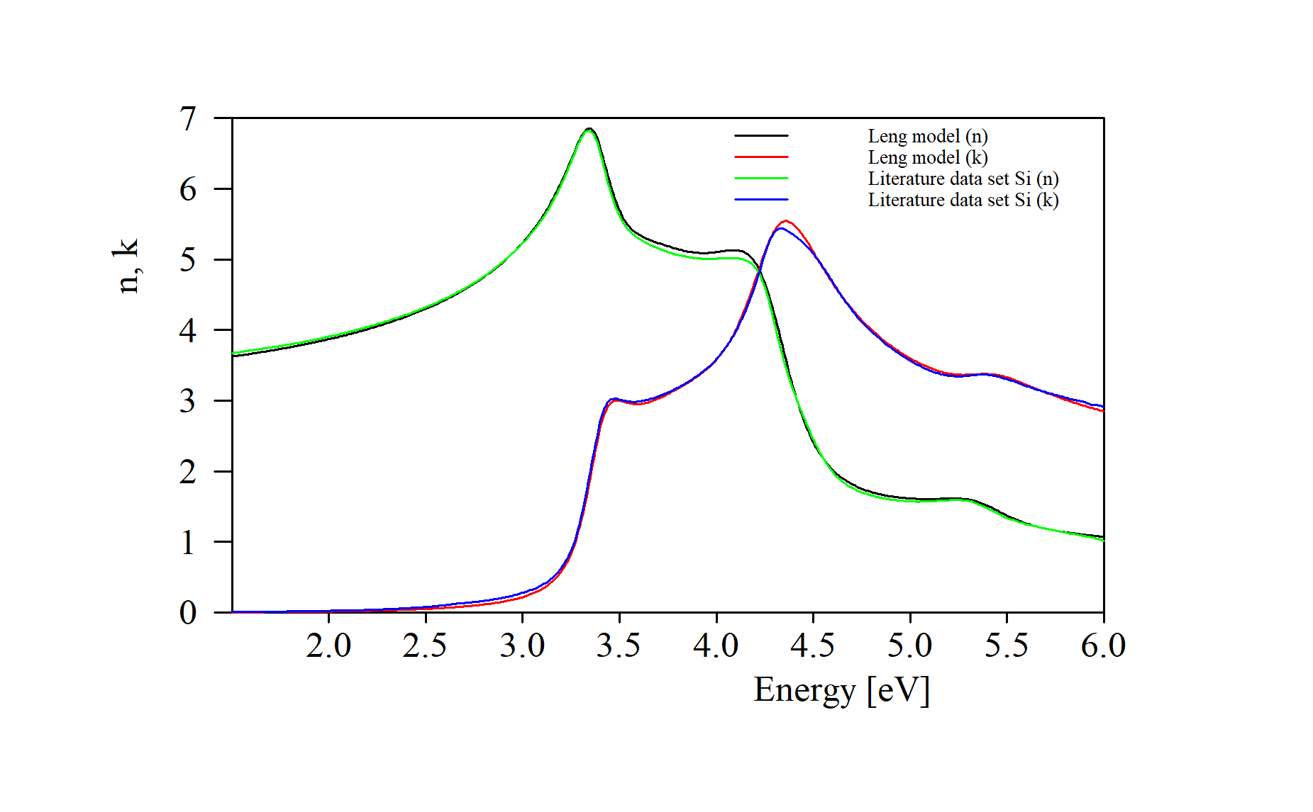
Warning: While the model works fine in the vicinity of strong spectral features (critical points in the joint density of states) it may generate non-physical n and k values in regions of small absorption.
BREIN: Actions/Delete selected record
Finally we have introduced a menu command (Actions/Delete selected record) to remove a record from the BREIN database. The action is – of course – password protected.
New optical functions
We have added optical functions which return statistical numbers based on cell values in the workbook or batch control windows. They are useful if you determine thickness profiles and want to display average thickness, minimum and maximum values, as well as standard deviation from the average.
The functions are explained here:
https://www.mtheiss.com/help/final/html/scout3/?workbook-and-batch-control.htm
Error messages in OLE automation
In object generation 4.97 we have implemented a new mechanism to pass error messages from SCOUT and CODE to OLE automation clients.
While it runs the OLE server (i.e. SCOUT or CODE) collects error messages in a list. We have introduced a view object (type ‘Error messages view’) to display the current list of error messages in a view.
Any OLE client (LabView, Excel, …) can retrieve information about the number of error messages, their type and text content. There is also a classification to separate critical errors and warnings. Once the OLE client has finished error handling it can clear the list in the OLE server.
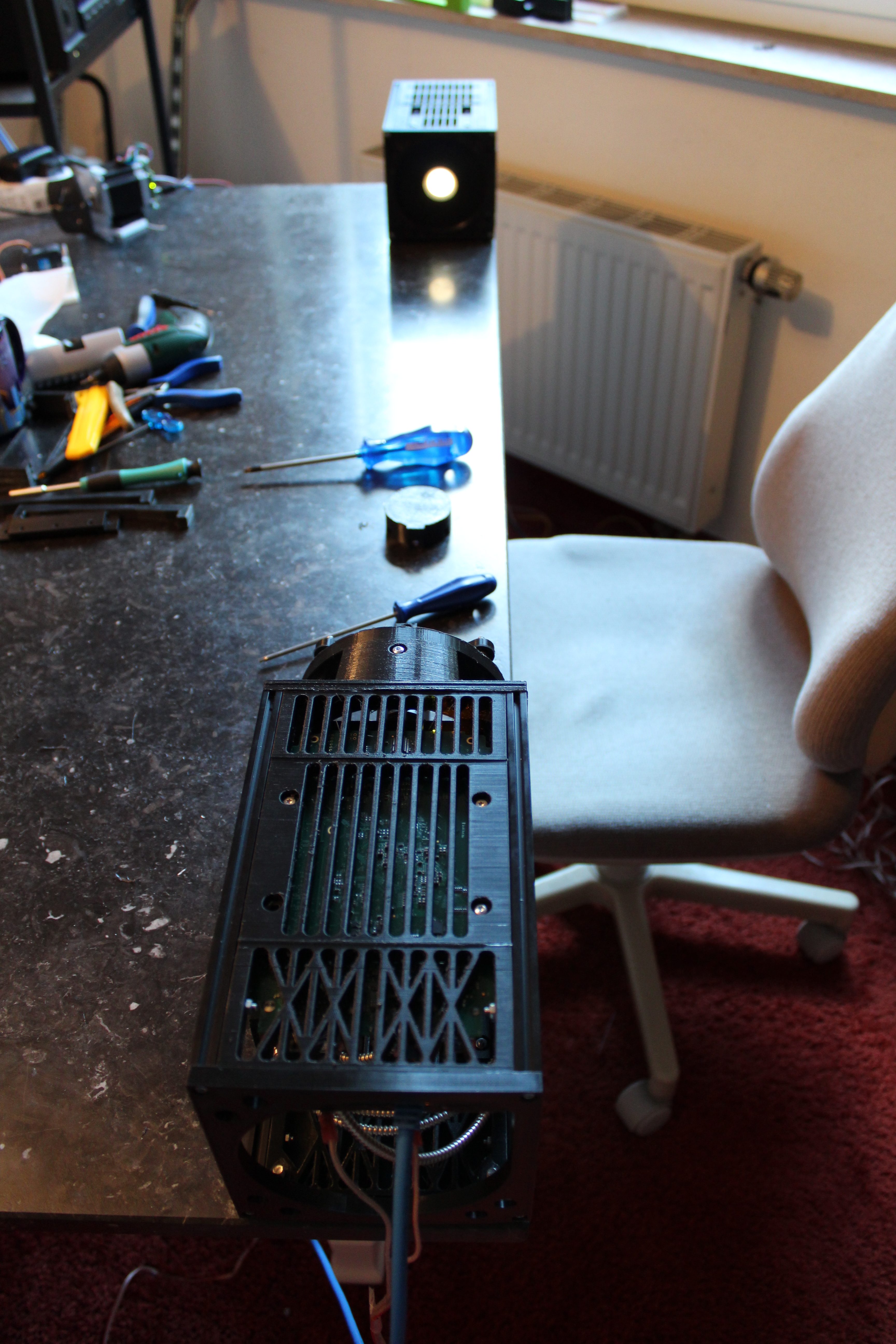
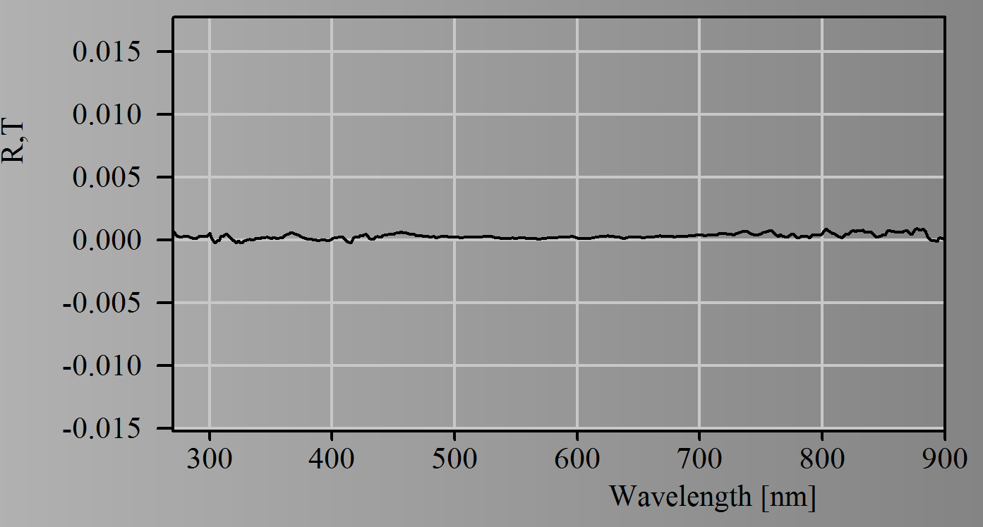
WOSP-LEDO – a new UV-Vis light source based on LEDs only
Our new WOSP-LEDO light source generates a homogeneous area of light emission, covering the spectral range 270 … 900 nm. It uses LEDs only – small power, long lifetime.
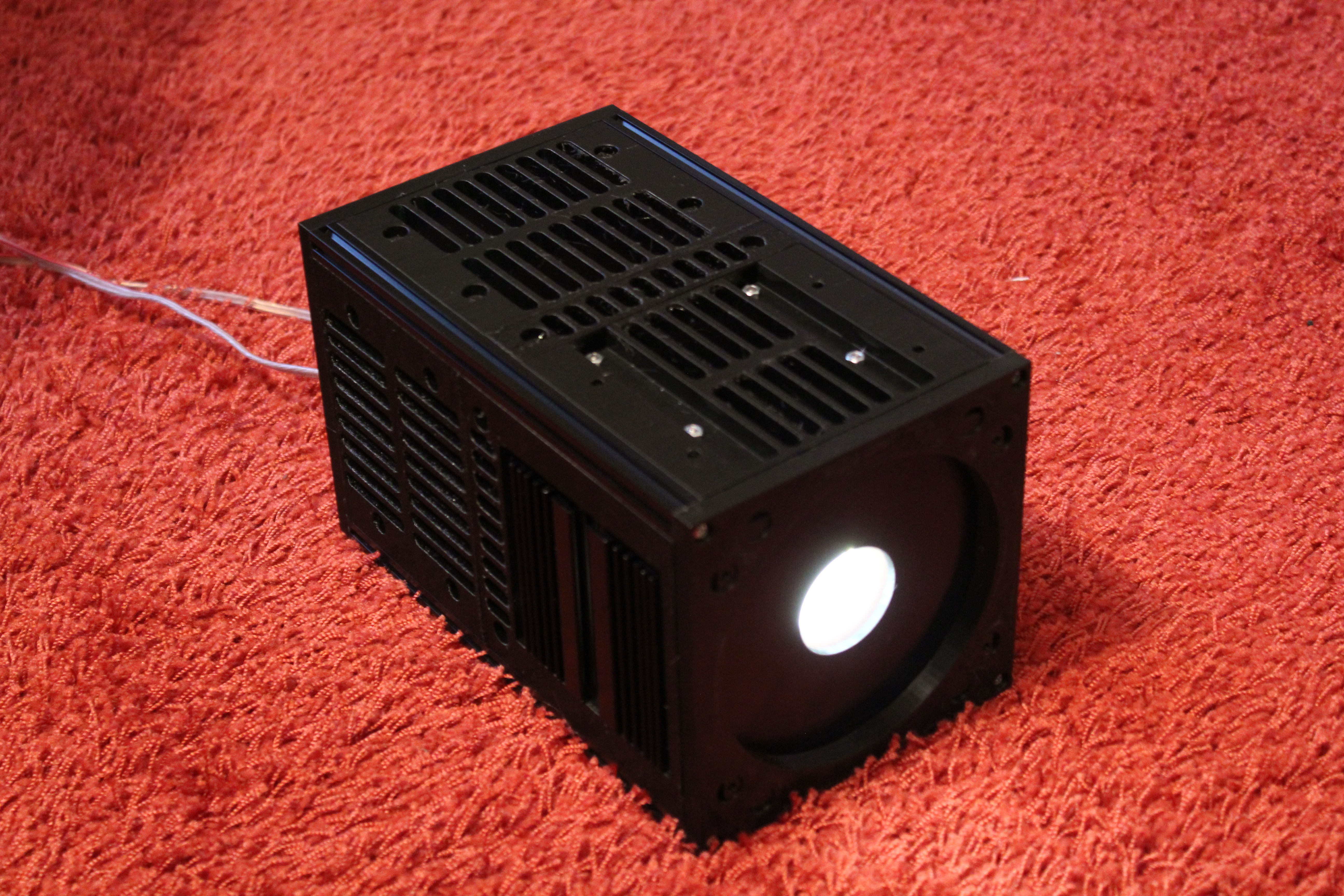
You can point a collimated field of view of an array spectrometer to the center of the light source and record transmittance or reflectance spectra in lab quality, within a fraction of the time a lab instrument would need.
The following transmittance spectra (100%, 0%, Schott Borofloat glass) have been recorded in less than 1 second, with a distance of about 1 m between light source and detector: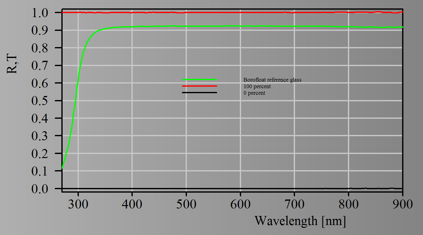
Zooms into the 0 and 100 percent spectra show excellent spectral quality:

New workbook functions
There are new script commands to write text and numbers to the workbook. The number to be written as well as row and column of the write action may be computed using user-defined expressions. You can refer to master parameters, fit parameters, optical functions and integral quantities in these expressions.
In the opposite direction, we have implemented new optical functions to compute average and standard deviation of rectangular blocks of cells, both in the workbook and the batch control window. As object names you have use the terms ‘workbook’ or ‘batch control’. The argument of the function call must specify the name of the worksheet as well as the start row and start column, and the end row and end column – all separated by commas.
Object export to workbook
In addition to optical constants and spectra, the menu command File/Report/Object data to workbook now (you need object generation 4.94) exports the layer stack definitions.
In CODE the integral quantities are added as well.