All posts by Wolfgang

Presentations with CODE

Object generation 3.98

We have been using CODE for a long time already to show interactive presentations about thin film optics. The related program features are now official parts of the software.

A CODE presentation is basically a sequence of configurations that provide the individual pages  of the presentation. There are some mechanisms to navigate through the presentation. If you maximize CODE and put it into presentation mode (key ‘p’ on your keyboard) you can show full screen presentations that look like Powerpoint. Inside, however, you are using fully functional CODE configurations with all slider and animation features.

There are view elements for easy navigation. You can have a table of contents providing direct access of every page (on the left side in the image below) and a control to jump to the next, previous or first page (upper right corner):

presentation_start

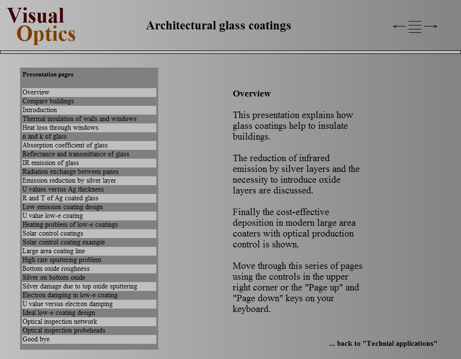
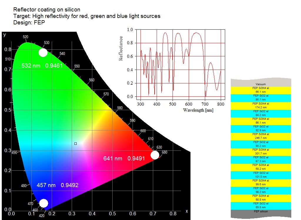
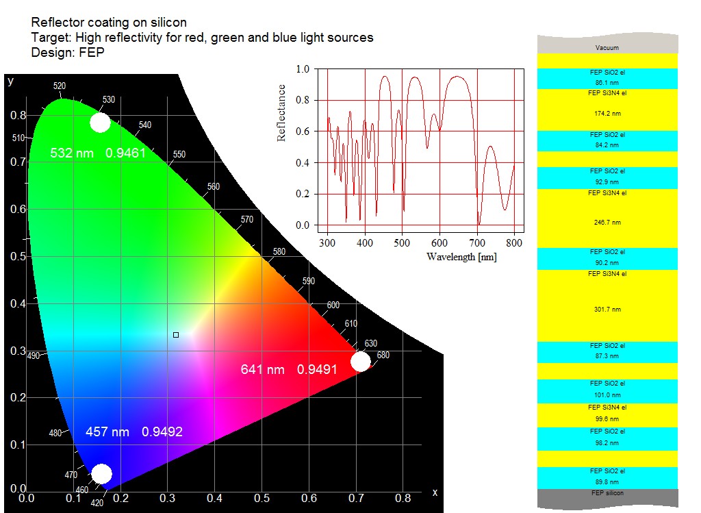
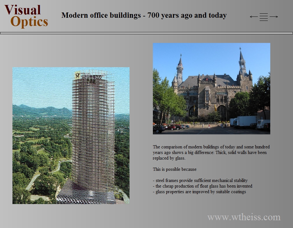
Your pages (=configurations files) can be either static

presentation_static_page

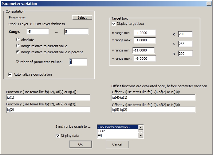
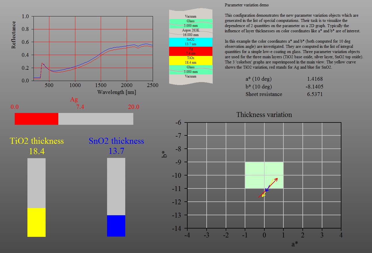
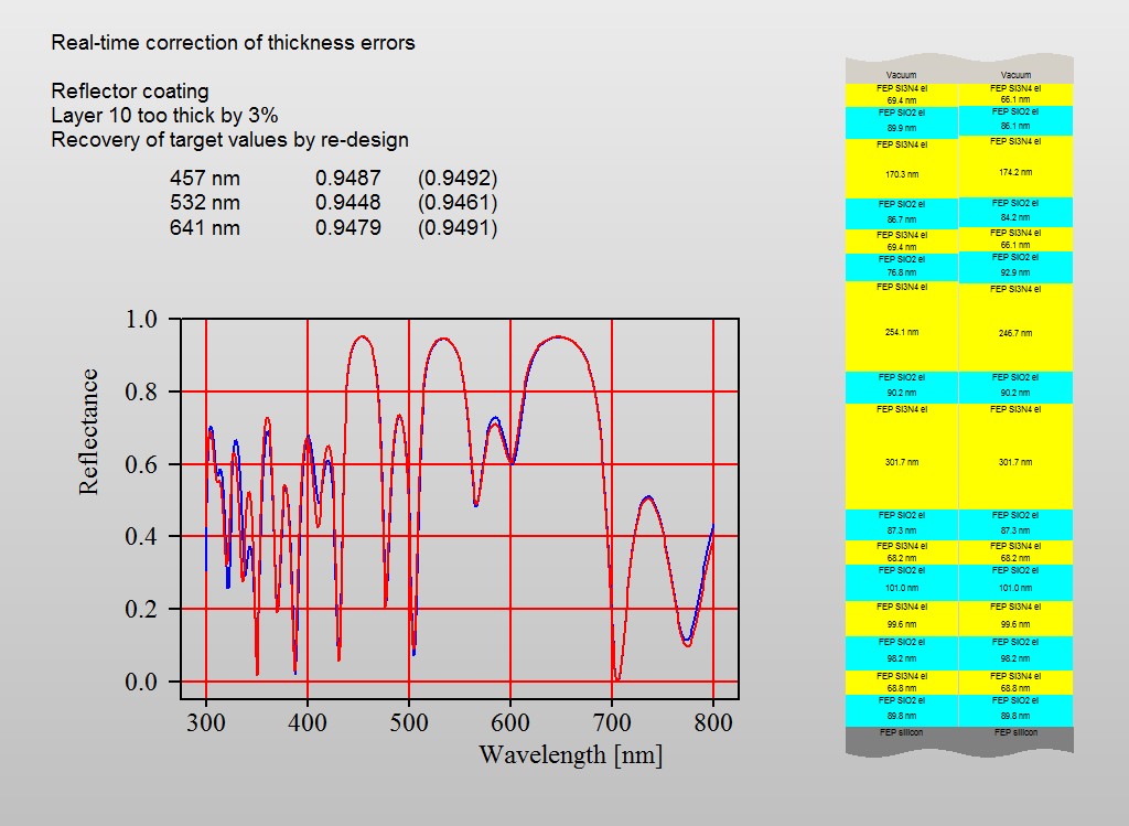
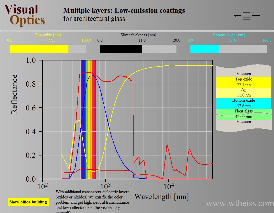
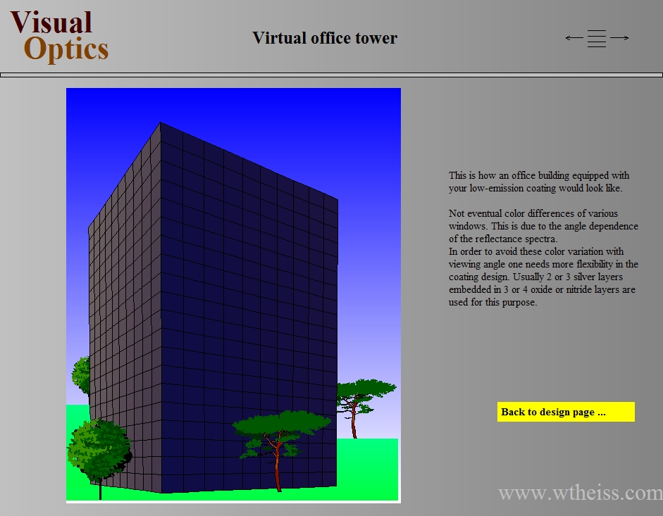
or dynamic, re-computing coating properties in real time while you move values by graphical sliders:

presentation_dynamic1

presentation_dynamic2

Here is the documentation of the new presentation feature. The online help system provides a link to a demo presentation that you can use to try it out yourself. You must have object generation 3.98 or higher.

Special computations: Parameter variation enhanced

CODE 3.98

The capabilities of ‘parameter variation’ objects in the list of special computations have been enhanced. You can now define ‘offset functions’ which are computed once before the parameter variation is executed. The example below discusses an application of this feature.

Suppose you are computing the dependence of color coorinates a* and b* on layer thicknesses. For each layer you generate an ‘arrow diagram’ showing how the position of the layer stack in the a*-b*-plane changes with thickness modifications. Superimposing 3 of such diagrams would give a graph like this:

originalUnfortunately the model does not perfectly reproduce the measured reflectance spectrum. As a result, the ‘measured’ color position is different from the simulated one. In this situation you might want to display the arrows at the ‘measured’ color position, believing that the direction and the size of the arrows will be similar there. A graph like this would show operators where they are with their real product and where they would go with thickness variations.

You can generate the desired offset the following way. Compute a* and b* of the simulated spectrum in the list of integral quantities as item 1 and 2, and compute the a* and b* of the measured spectrum as items 4 and 5. In function definitions you can refer to these numbers as iq(1), iq(2), iq(4) and iq(5), respectively. The dialog for the first parameter variation object (modifying the TiO2 layer thickness) would look like this:

sc_parameter_variation_dialog

Defining similar offsets for the other two layer thickness variation objects you will get a shifted arrow graph, centered at the color position of the measured reflectance:

shiftedObviously, you should use this feature only in cases where you are sure that the applied offset is justified and does not lead to wrong conclusions.


BREIN prediction window gets measured spectra

Measured spectra are now passed to the prediction window. In order to get this working the prediction configuration has to have spectrum objects with the same names as the Bright Eye which triggers the prediction update. Only the spectra recorded at the “trigger position” are sent.

In order to use this feature you have to get brein.exe and bright_eye_traverse.exe programs generated after September 13, 2014.

Here is the BREIN download page.

BREIN prediction feature

There is a new BREIN tab called ‘Prediction’. It predicts the performance of a final product based on the current state of the production.

The mechanism behind is the following: After the final traverse analysis the values of the fit parameters are passed to a CODE configuration which produces the prediction graph. Typically the numbers are layer thicknesses – this way the predicting CODE program knows the current layer stack and can compute the performance of any glazing product that includes the actual coating. So the operators can take a look at the final product including gas fillings and second or third panes.

The prediction is done for a single traverse position. It is triggered by the arrival of new results for this position only.

More flexible layer stack view

Introduced with object generation 3.97

Visualizing a layer stack in views is now more flexible. Instead of representing each layer as a rectangle of constant height (i.e. the same height for all layers) the graph can now better visualize the proportions by drawing the rectangles with heights proportional to the thickness of the layer.

The graphs below show the difference. Up to now layer stack views looked like this:

16_3_design_0

Now you can have this:

16_3_design

This kind of drawing makes it much easier to compare layer stacks:

16_3_comparison

The new kind of drawing is activated by a click on the layer stack in the view. You will be asked for the thickness that the height of the base rectangle should represent. The value must be specified in micrometers – if you set a value to 0.075 the base rectangle shows 75 nm of the stack.

Since layer thickness values in stacks with thin films and (incoherent) thick layers are very different, it is not possible to see thick layers and thin films in one graph. Thin films with thicknesses 100000 times smaller than thick layers will simply not be visible (like in real life). If you still want to show the thin film part of the stack with the new feature you have to use 2 layer stacks: one for the thin film coating alone and the second one for the complete layer stack. In this case you have to insert the coating as ‘included layer stack’ in the second one.

SPRAY surface textures

SPRAY is a powerful tool to optimize the performance of solar cells. In order to simplify the modeling of crystaline silicon PV modules we have added an easy way to define macroscopic surface texture. This new feature can be used for both the covering glass and the Si wafer surface.

A PV module consists of a silicon wafer with top and backside contacts:

wafer spray

The wafer is embedded in EVA:

wafer spray packed

The EVA is covered by glass which gives mechanical strength and protection for the next 30 years. In order to maximize the generation of electric power one may introduce an

  • anti-reflection (AR) layer between silicon and EVA
  • AR layer between glass and air
  • surface texture of the silicon wafer
  • surface texture of the cover glass
  • diffusely reflecting white backside
  • low-absorptive cover glass

In order to find out how much the PV output is increased by these improvements one can perform realistic ray-tracing computations with SPRAY. This can save a lot of experimental work and costs. SPRAY performs 3D spectral ray-tracing and records where how much radiation is absorbed. It can, for example, output the spectrum of absorbed light in the wafer

wafer spray result1


as well as the spatial distribution of absorbed light:

wafer spray absorption depth profile

The graph below shows a comparison of the absorbed fraction with and without a simple AR coating (a single SiN layer) between silicon and EVA:

wafer spray simple SiN AR


The modeling of macroscopic surface textures is now much easier using the new object type ‘Periodic surface texture’. This is a rectangle with a regular surface pattern in the x- and y-direction. You can set the periodicities in both directions and select a pattern type. Depending on the type of texture you can set additional parameters in the object dialog:

clip0001


The available textures are the following:

Sine profile

clip0002


Pyramids
clip0003
Inverted pyramids
clip0004
Cones
clip0005
Inverted cones
clip0006
 
Half spheres
clip0007
 
Inverted half spheres
clip0008

Improved start behavior

If BREIN was started after a long break during which a large number of results have been generated, the software was not responsive for a long period of time (because it was reading many result files). You can now limit the number of result files to be processed during one timer event (which happens every second). A number of 20 is reasonable and has been set as default value. You can change this choice in the Settings submenu.