Starting with object generation 5.11 we have introduced a new spectrum type called ‘Rp/Rs’. If you select this option the spectrum object computes the ratio of the intensity reflectance for p-polarized light and s-polarized light. This ratio can be directly fitted to experimental data if your measurement system produces this quantity as final result.
Category Archives: Optical modeling
Tolerated intervals for integral quantities
Design targets for color values or other integrated spectral values may not always be well-defined numbers. You can also search for designs where color values stay within tolerated boundaries, but it does not matter where exactly.
Such design situations can be handled in CODE using so-called ‘penalty shape functions’. However, the use of this concept turned out to be rather complicated.
We have now (starting with version 5.02) introduced a very easy definition of tolerated intervals for integral quantities: Instead of typing in the target value you can define an interval by entering 2 numbers with 3 dots in between, like ’23 … 56′ or ‘-10 … -8’. If the integral value lies within the interval its contribution to the total fit deviation is zero. Outside the interval the squared difference between actual value and closest interval boundary is taken, multiplied by the weight of the quantity.
Leng model for optical constants
We have implemented (starting with object generation 4.99) the Leng oscillator which has been developed to model optical constants of semiconductors. As shown in the original article (Thin Solid Films 313-314 (1988) 132-136) it works well for crystalline silicon:
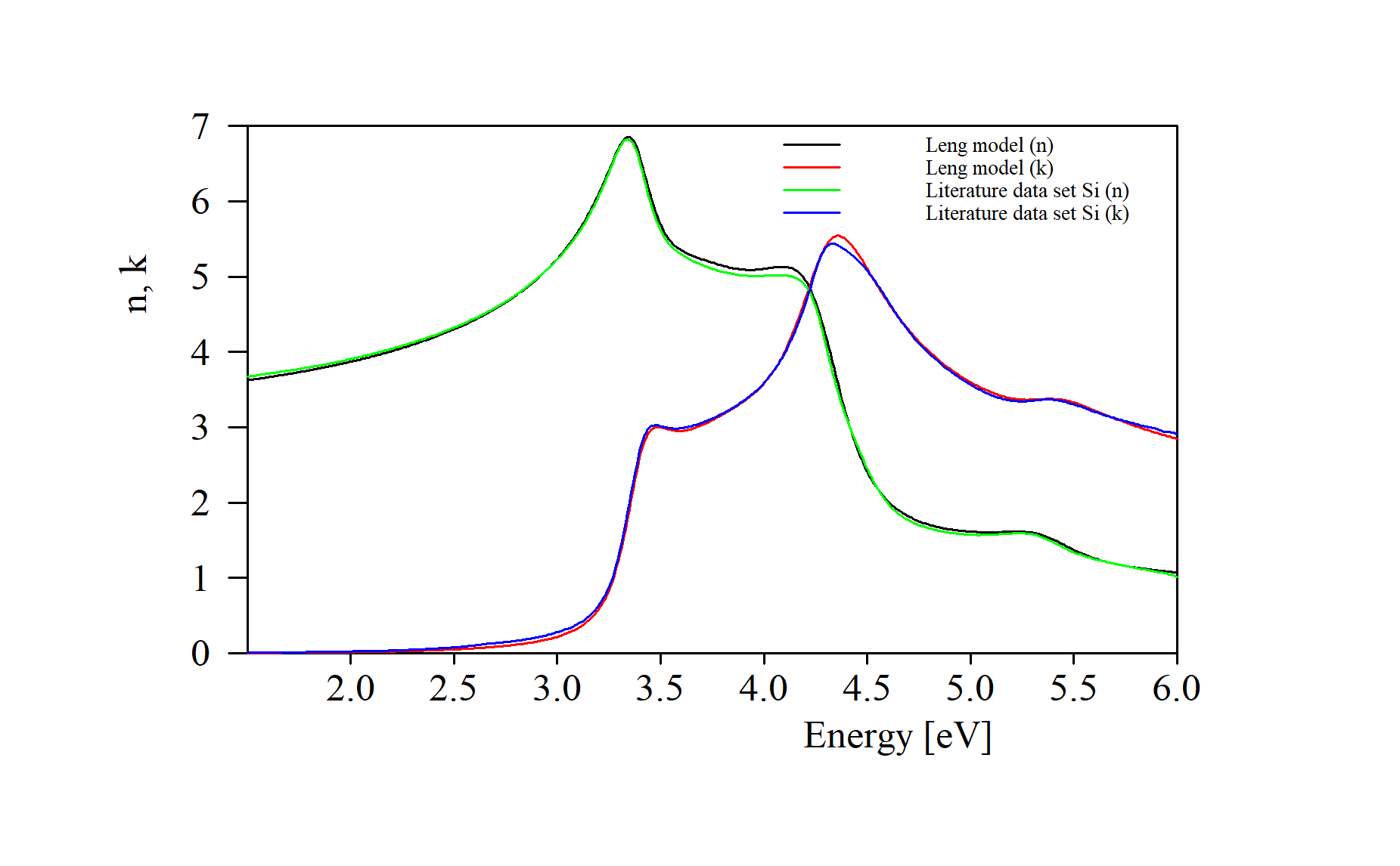
Warning: While the model works fine in the vicinity of strong spectral features (critical points in the joint density of states) it may generate non-physical n and k values in regions of small absorption.
Bugfix master model
With version 4.56 we have removed a bug in master models for optical constants. Saving a successful model and re-loading it could lead to a strange mix-up of parameter values in some situations, leaving the poor user with a useless configuration. We recently taught CODE and SCOUT to correctly count master and slave parameters – saving and loading should work now.
Gradient?
How do I describe a gradient of optical constants?
A gradient of optical constants can be implemented in an optical model using the layer type ‘concentration gradient’.
The strategy is this:
Define an effective medium, i.e. a mixture of 2 materials, using one of the simple effective medium objects Bruggeman, Maxwell-Garnett or Looyenga. The best choice for gradients is Bruggeman, also known as EMA. The only parameter to describe the topology of the mixture is the volume fraction.
In the next step, insert a concentration gradient layer into the layer stack and assign the effective medium material to it. The gradient will be described by a user-defined function that defines the depth dependence of the volume fraction from the top of the layer to the bottom. Select the layer and use the Edit command to access the formula definition window.
Finally, you go back to the layer stack definition window and specify how many sublayers should be used to sample the gradient. Be careful not to take too many sublayers – this could increase the computational times a lot. On the other hand, be careful not too ‘undersample’ the gradient – if you increase the number of sublayers by 1 the spectra should not change significantly.
Please consult the manual for further details …
Roughness
How do I describe surface roughness?
Roughness can be taken into account in different ways in optical models for thin films.
The easiest way is to replace the sharp interface between two materials by a thin layer with mixed optical constants. This is a good approach for roughness dimensions clearly below the light wavelength. Mixed optical constants can be computed using an effective medium model. The Bruggeman formula (also known as EMA – effective medium approximation) is a good choice (please read the remarks below). Start with a very thin intermediate layer (e.g. 2 nm) and select its thickness as fit parameter. The volume fraction of the effective medium model should be an adjustable fit parameter as well.
An advanced version of this kind of roughness modeling is to use a concentration gradient layer. This type of layer can describe a smooth transition between adjacent materials. The depth dependence of the volume fraction can be expressed by a user-defined formula with up to 6 parameters that can be fitted.
A warning must be raised using effective medium models to describe roughness effects. All effective medim models in our software are made for two phase composites which are isotropic in three dimensions. They are not valid for surface roughness effects. To apply these concepts anyway can be justified by saying that there is no reasonable alternative and that it is very common to do so …
Describing rough metal surfaces with an effective medium model may be a little tricky. This is especially true for silver. Inhomogeneous metal layers can be efficient absorbers with very special optical properties, and effective medium approaches can be very wrong – please read SCOUT tutorial 2 about this.
The roughness described by effective medium layers does not lead to light scattering but modifies the reflectance and transmittance properties of the interface between the adjacent materials. Light scattering at heavily rough interfaces can be taken into account in a phenomenological way in cases where the detection mechanism of the spectrometer system does not collect all the scattered radiation. You can introduce a layer of type ‘Rough interface’ which scales down the reflection and transmission coefficients for the electric field amplitude of the light wave. The loss function is a user- defined function which may contain 2 parameters C1 and C2 which are fit parameters. In addition, the symbol x in the formula represents the wavenumber.
The expression C1*EXP(-(X/C2)^2), for example, would describe an overall loss by a factor C1 and an additional frequency dependent loss which is large for small wavelengths and small for large wavelengths. This kind of approach has turned out to be satisfying in several cases.
How accurate?
How accurate are the results when I use optical modeling?
This is hard to tell, and it depends on many details. So there is no general answer to this question.
A good optical model should use the lowest possible number of parameters. If you have too many parameters in the model they may be correlated in a way that raising one parameter value and decreasing another leads to the same optical spectra. In this case the parameter values are more or less arbitrary, and the accuracy is very low.
The result of a parameter fit depends very much on the information contained in the measured data. If you want to determine a layer thickness, for example, you must have measured contributions of radiation which has seen the bottom of the layer, i.e. which has travelled through the layer at least once. If that is not the case in the spectral range that is accessible to you, you will never be able to get the thickness of the layer.
Any real result?
Can I get anything real out of a model?
Yes, of course. If your model is good, and your spectra do contain enough information, the parameter values reflect the real values as good as they can.
Please have in mind that in many cases talking about ‘real values’ is using a model in itself. If you ask for the real value of a layer thickness, for example, your question implies that there is something like a layer with a top and a bottom end. You ignore the atomic structure and surface roughness effects, or, if not, you apply (at least in your mind) a certain roughness averaging procedure.
Why optical modeling?
Why do I have to use optical modeling?
Optical modeling is a very clean and transparent way of analyzing measured optical spectra. If the model is done in a good way it has exactly the parameters that you want to know, such as film thicknesses, band gaps, amounts of impurities or carrier concentrations.