
Introduced with object generation 3.97
Visualizing a layer stack in views is now more flexible. Instead of representing each layer as a rectangle of constant height (i.e. the same height for all layers) the graph can now better visualize the proportions by drawing the rectangles with heights proportional to the thickness of the layer.
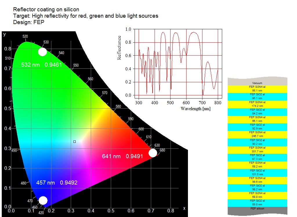
The graphs below show the difference. Up to now layer stack views looked like this:
Now you can have this:
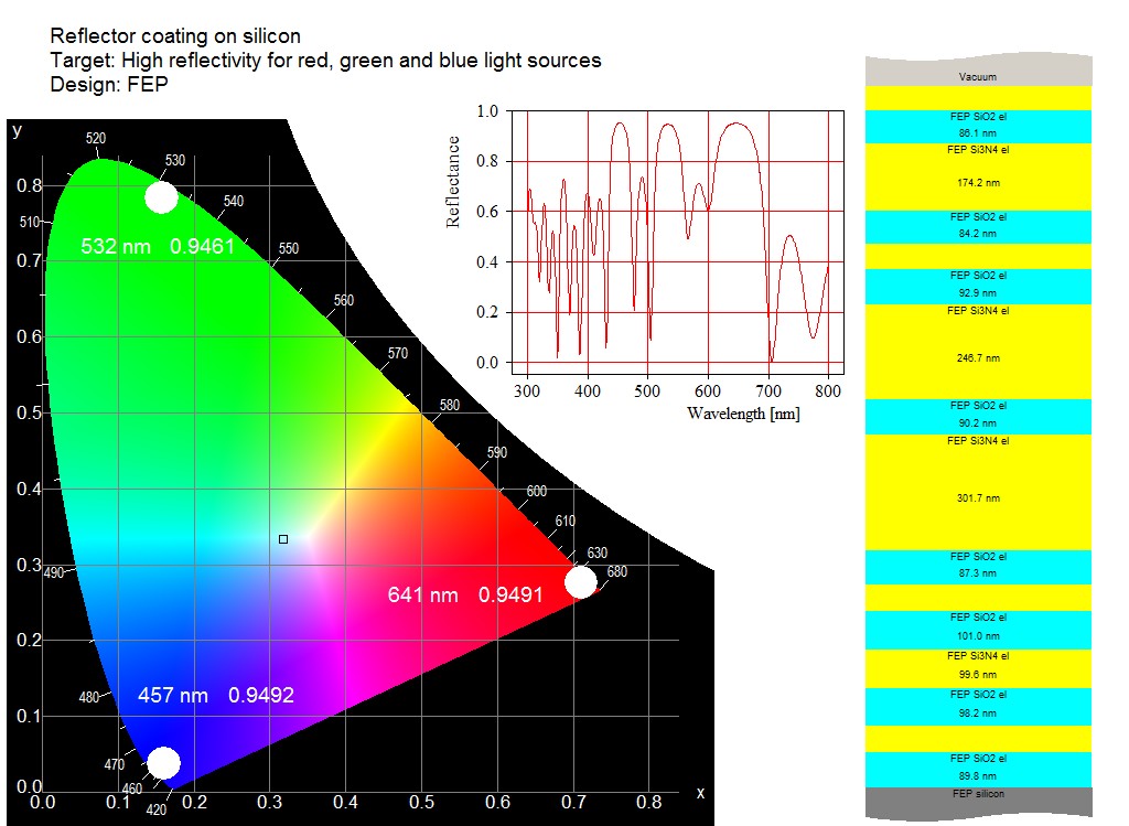
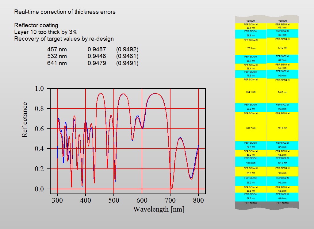
This kind of drawing makes it much easier to compare layer stacks:
The new kind of drawing is activated by a click on the layer stack in the view. You will be asked for the thickness that the height of the base rectangle should represent. The value must be specified in micrometers – if you set a value to 0.075 the base rectangle shows 75 nm of the stack.
Since layer thickness values in stacks with thin films and (incoherent) thick layers are very different, it is not possible to see thick layers and thin films in one graph. Thin films with thicknesses 100000 times smaller than thick layers will simply not be visible (like in real life). If you still want to show the thin film part of the stack with the new feature you have to use 2 layer stacks: one for the thin film coating alone and the second one for the complete layer stack. In this case you have to insert the coating as ‘included layer stack’ in the second one.