
Reflectance spectra of the TohoSpec3100 system can now be imported both in SCOUT and CODE.
Category Archives: CODE
Check-out managed license
You can now check-out a managed license for offline use. The typical scenario is that you plan to travel with your laptop and expect to have no internet connection for a while. In this situation you can use the menu command “?/Check out managed license for offline use” while you still have a connection to the internet. You have to specify the number of hours for which you will be offline. During this time you can work without connection to the license server.
The license server blocks your license for the indicated offline time for other users. If your license is one license of a pool shared by several users act responsibly and declare reasonable offline periods only.
If your offline time is over earlier than expected you can use the menu command “?/Un-do managed license check-out” to tell the server that you are online again. Your license will then be available for other users if you do not use if for some minutes.
Analysis of color sensitivity
If you would like to check what color difference a thickness change of a layer in a stack may cause you can do that quite easily with a new feature of ‘color fluctuation’ objects. These integral quantities compute, for thickness fluctuations defined in the layer stack, the size of the ‘color cloud’ that you can expect when producing the stack many times.
Selecting an object of this type in the list of integral quantities, you can now use the menu command ‘Export data’ to generate a *.csv file with a table of color values that you get when the layer thickness values are individually modified. The files can be immediately opened by Excel, for example. Here is an example:

New script commands
In order to realize some new user interface options in views, we have introduced some new script commands. The available commands are described here.
New version of Live.exe tool
A new version of live.exe is available here. The new version makes it very easy to migrate your software from one computer to another.
Copy live.exe to your program directory (like c:\my_software\code\) and start it. Click on the button ‘Generate backup folder’ – the program lets you select a destination in your network and then backups the complete program folder and your application data, including your passport file. You should execute this backup function from time to time to save your software package. The destination folder should not be on the same drive as your original installation.
In order to install the software on a new computer you must make the backup folder accessible for the new machine. Then start live.exe in the backup folder and click on ‘Install software on this computer’. This action will do the installation for you and your software should now run on the new PC.
Note the following exceptions:
- If your software is protected by a USB dongle you must install the dongle driver on the new machine first. The dongle driver is available here.
- If your software is protected by activation you need to obtain a new passport file from us.
tec5 import routine
Object generation 3.98
An import routine for tec5 textfiles has been implemented.
Presentations with CODE
Object generation 3.98
We have been using CODE for a long time already to show interactive presentations about thin film optics. The related program features are now official parts of the software.
A CODE presentation is basically a sequence of configurations that provide the individual pages of the presentation. There are some mechanisms to navigate through the presentation. If you maximize CODE and put it into presentation mode (key ‘p’ on your keyboard) you can show full screen presentations that look like Powerpoint. Inside, however, you are using fully functional CODE configurations with all slider and animation features.
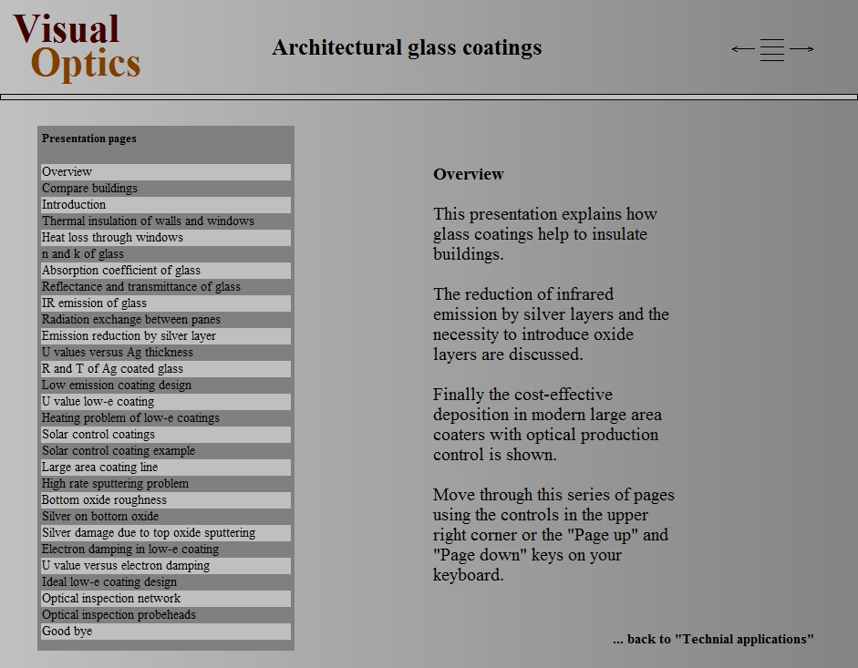
There are view elements for easy navigation. You can have a table of contents providing direct access of every page (on the left side in the image below) and a control to jump to the next, previous or first page (upper right corner):
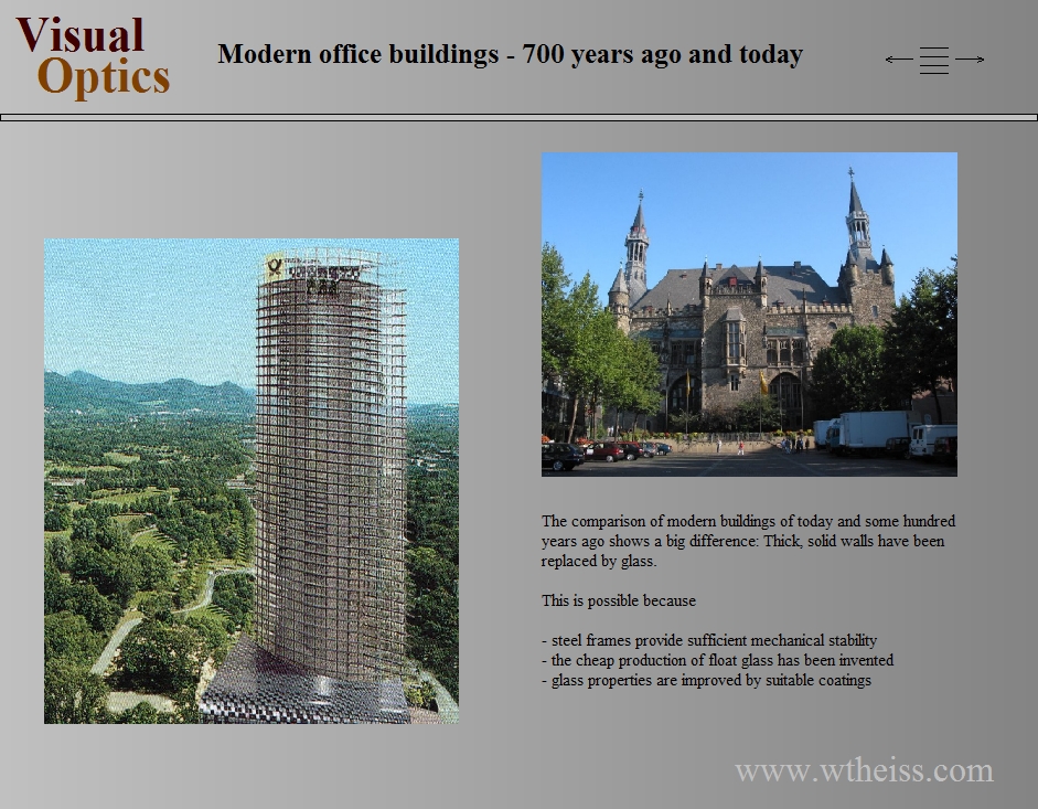
Your pages (=configurations files) can be either static
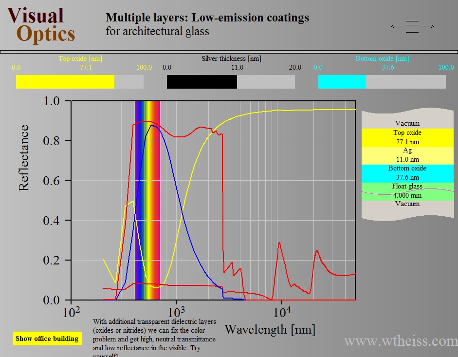
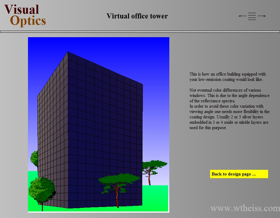
or dynamic, re-computing coating properties in real time while you move values by graphical sliders:
Here is the documentation of the new presentation feature. The online help system provides a link to a demo presentation that you can use to try it out yourself. You must have object generation 3.98 or higher.
PDF export improved
Problems displaying some view elements (layer stack view, background, color gradients) in PDF documents have been removed.
Special computations: Parameter variation enhanced
CODE 3.98
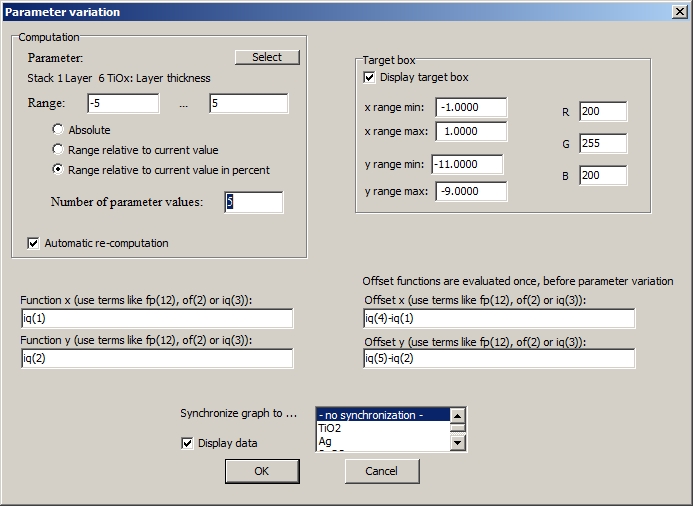
The capabilities of ‘parameter variation’ objects in the list of special computations have been enhanced. You can now define ‘offset functions’ which are computed once before the parameter variation is executed. The example below discusses an application of this feature.
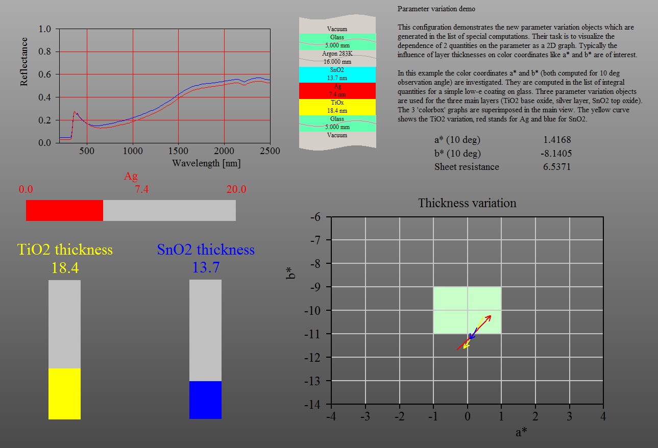
Suppose you are computing the dependence of color coorinates a* and b* on layer thicknesses. For each layer you generate an ‘arrow diagram’ showing how the position of the layer stack in the a*-b*-plane changes with thickness modifications. Superimposing 3 of such diagrams would give a graph like this:
 Unfortunately the model does not perfectly reproduce the measured reflectance spectrum. As a result, the ‘measured’ color position is different from the simulated one. In this situation you might want to display the arrows at the ‘measured’ color position, believing that the direction and the size of the arrows will be similar there. A graph like this would show operators where they are with their real product and where they would go with thickness variations.
You can generate the desired offset the following way. Compute a* and b* of the simulated spectrum in the list of integral quantities as item 1 and 2, and compute the a* and b* of the measured spectrum as items 4 and 5. In function definitions you can refer to these numbers as iq(1), iq(2), iq(4) and iq(5), respectively. The dialog for the first parameter variation object (modifying the TiO2 layer thickness) would look like this:
Defining similar offsets for the other two layer thickness variation objects you will get a shifted arrow graph, centered at the color position of the measured reflectance:
 Obviously, you should use this feature only in cases where you are sure that the applied offset is justified and does not lead to wrong conclusions.
Bug fix related to default font
The font for graphics and text in the main view was not always properly set after loading a configuration. This has been fixed.